Linear Regression

The linear regression model is one of the most popular models in machine learning for performing estimation ( predicting the values of a quantitative variable based on predictors ). It is a parametric technique - the model must find the best parameters based on the data -. This technique is used to fit the relationship between a numerical variable $Y$ ( dependent variable ) and a set of predictors $x_1, x_2,...x_n$ – independent variables.

We assume that $x$ and $y$ are not independent, meaning that knowledge of $x$ improves the understanding of $y$. Therefore, there is a correlation between $x$ and $y$. As a reminder : the more a variable $x$ is correlated ( positively or negatively ) with variable $y$, the more important it is for our model as we say it is « discriminative ». – see the chapter on ( correlation ).

Linear regression only accepts numerical predictors, meaning quantitative variables or qualitative variables that have been transformed through either one-hot encoding or through the process of discretization of categorical variables.

note

Some of the diagrams and concepts presented here are inspired by the Machine Learning course by Andrew Ng, a program created in collaboration between Stanford University Online Education and DeepLearning.AI, available on Coursera. Find the original course here: Machine Learning by Andrew Ng.

Single Predictor

The hypothesis is that the following function estimates the relationship between the predictor $x$ and the resulting variable $y$ :

$$\hat{Y} = b + w * x$$

This function corresponds to the equation of a line where $w$ represents the slope of the line, and $b$ is the y-intercept.

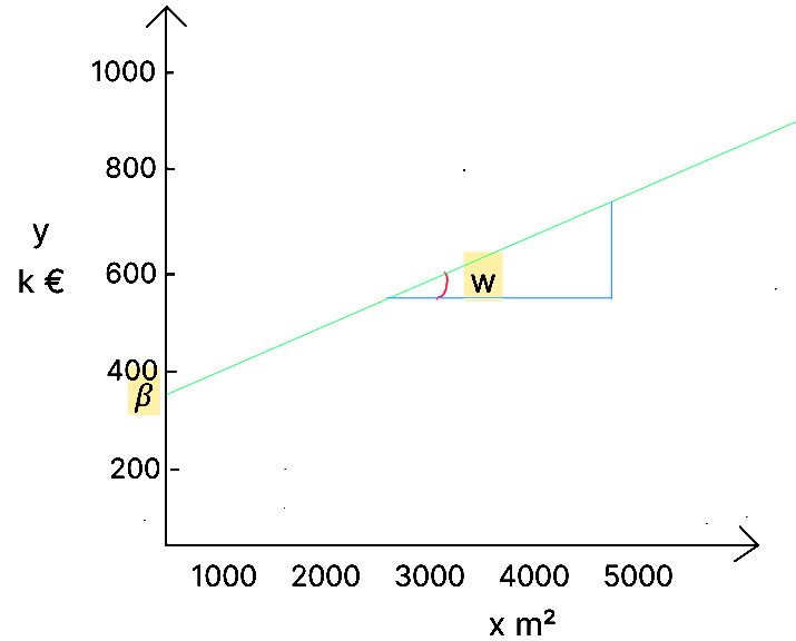
The data allows us to understand the relationship between the dependent variable and the independent variables, i.e. to estimate the coefficients and quantify the noise $ϵ$.

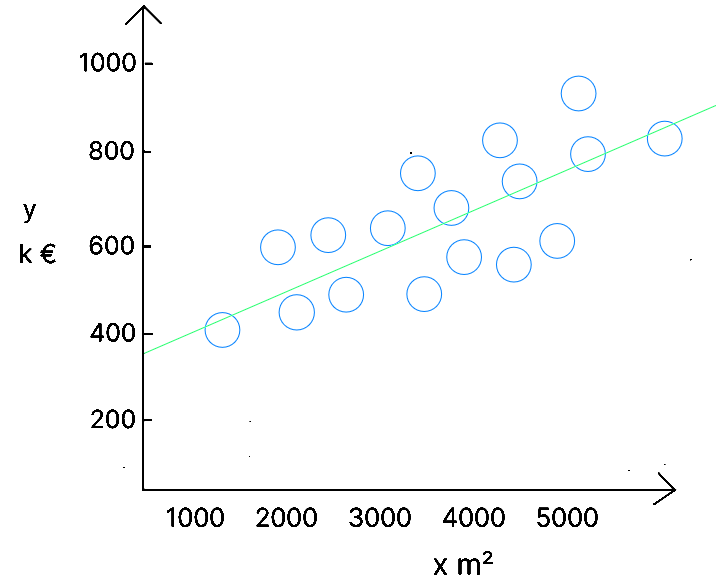
Let’s take the following data representing the size of a house ($x$) and its sale price ($y$):

$n$	Size in m² $x$	Price (k) $y$
1	2104	400
2	1416	232
3	1524	315
4	852	178
…	…	…
47	3210	870

The goal of the algorithm is to obtain a model that can be represented by the line minimizing the differences between the real values ( the bubbles ) and the predicted values ( the line ). Based on the values of $x$, the algorithm will define $\hat{Y}$ ( which is not equal to $y$ ), by finding the values of $b$ ( the origin of the line – if there is no house, there is still a base value, such as the land ) and $w$ – the slope of the line.

Error or Noise

As we discussed in supervised learning, the goal of a prediction model is to define a generalizable rule. This means avoiding a model that is either underfitting or overfitting. A generalizable rule means that the model does not perfectly fit the training data to ensure it can be applied to new data and achieve a good score.

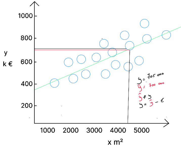
Therefore, we will never obtain a model that makes perfect predictions. We will always have what we call an error - denoted as $ϵ$ - ( a difference between the predicted value $\hat{Y}$ and the actual value $Y$ ), and our goal as data scientists is to select the model - during the evaluation phase - that minimizes this error.

For a given data point $n_3$, we know $x$ corresponds to $4500 m²$, and we know $y$ is equal to €705,000. After applying our algorithm to the data, a model was created, represented by the line $\hat{Y} = b + w * x$. If we look at the predicted value for $n_3$ - represented by the red line, i.e. the intersection between our model's line and the m² value - we observe that our model gives a price of €700,000. Thus, there is an error of €5,000 in the prediction. This error is expected because our model had to adapt to all the data. This is why it is important to understand that $\hat{Y} ≠ y$ but $\hat{Y} = y + ϵ$ ( the error ). In our case: $\hat{Y} = y + (-5000)$.

The equation for simple linear regression $y = \hat{Y}$ should therefore be rewritten as :

$$y = b + w * x + ϵ$$

or

$$\hat{y} = b + w * x$$

or also:

$$\hat{y} = f_{w,b}(x)$$

Prediction function in Python for simple regression

def predict(x, w, b):
    p = x * w + b
    return p

Cost Function

In order to perform learning, we first divided our data into ** explanatory variables ( $x$ ) and the target variable ( $y$ )**, and when we build a linear regression model; we have values for both $x$ and $y$. The goal of our model $\hat{Y} = b + w * x$ is therefore to define $w$ and $x$.

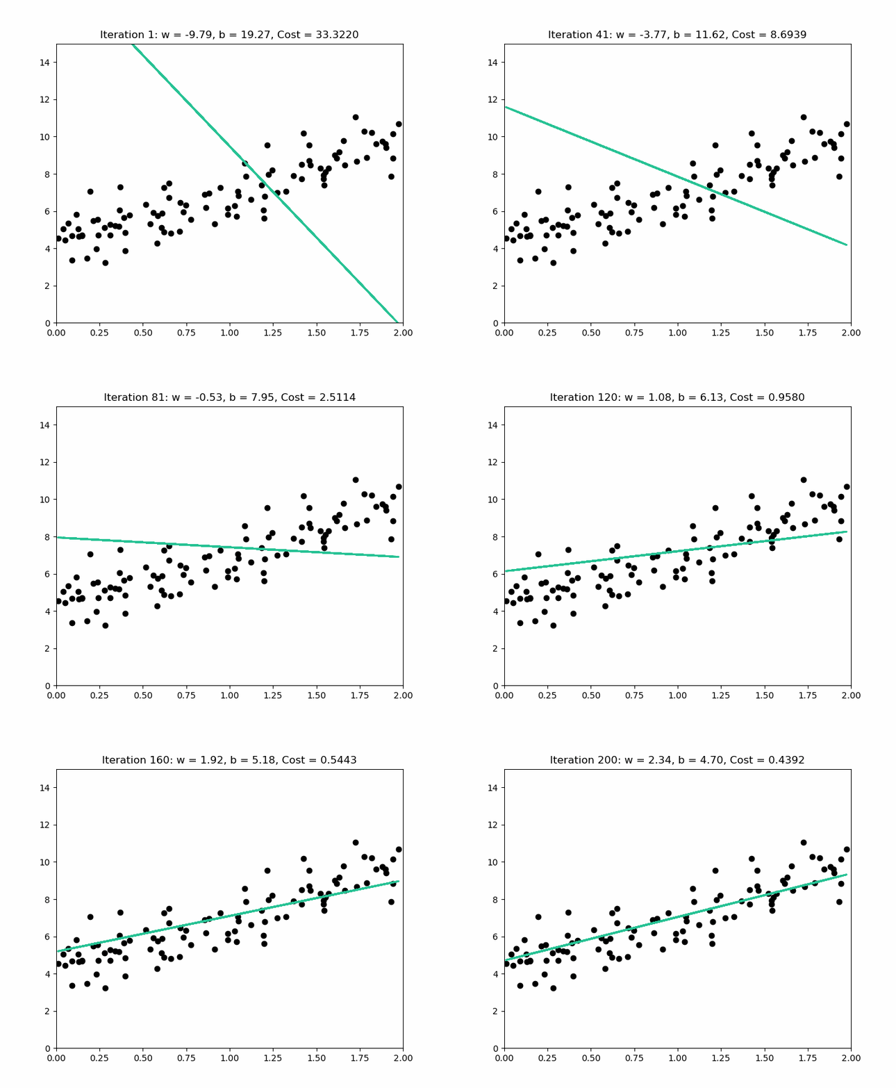
How does our algorithm find the values of $w$ and $x$ ? It's simple ! As we mentioned earlier, during the learning step, the machine considers the $x$ and $y$ values from the training set to identify $w$ and $x$ by iterating based on a cost function that it minimizes.

The algorithm uses the function $\hat{Y} = b + w * x$. It replaces $x$ with the training data values and randomly assigns initial values to $b$ and $w$. It then calculates the error weight of the model based on these initial values for $b$ and $w$, analyzing the differences between the $y$ values and the $\hat{Y}$ values for each record. Then, to find the local optimum - that is, the values of $w$ and $b$ that minimize the cost (the error) -, it uses an optimization algorithm : gradient descent.

The goal of the cost function is to minimize $\hat{y} - y$ for each record. By convention, in machine learning, the cost function is denoted as $J$.

Thus, the goal of the cost function is to minimize errors, which can be written as : $J(w, b) = \min \sum_{i=1}^n (\hat{y}^{(i)} - y^{(i)})^2$, where the error is squared to prevent positive and negative errors from canceling each other out.

However, this formula is incomplete because we want to minimize the average error. To do this, we multiply the sum of the errors by $\frac{1}{m}$, resulting in : $J(w, b) = \min \frac{1}{m} \sum_{i=1}^n (\hat{y}^{(i)} - y^{(i)})^2$ in order to normalize the cost function with respect to the number of records.

In literature, we find an adaptation of this function to simplify the calculation of the derivative of the cost function. Indeed, to find the local optimum ( the cost function that minimizes the errors ), we use the gradient descent algorithm, which calculates the derivative of the cost function to determine at each iteration whether to increase or decrease $b$ and whether to decrease or increase $w$.

Thus, the cost function is written as :

$$J(w, b) = \min \frac{1}{2m} \sum_{i=1}^n (\hat{y}^{(i)} - y^{(i)})^2$$

and we could replace $\hat{y}$ with ($w \cdot x^{(i)} + b$), which gives :

$$J(w, b) = \min \frac{1}{2m} \sum_{i=1}^n ((w \cdot x^{(i)} + b) - y^{(i)})^2$$

or

$$J(w, b) = \min \frac{1}{2m} \sum_{i=1}^n (f(w,b)x^{(i)} - y^{(i)})^2$$

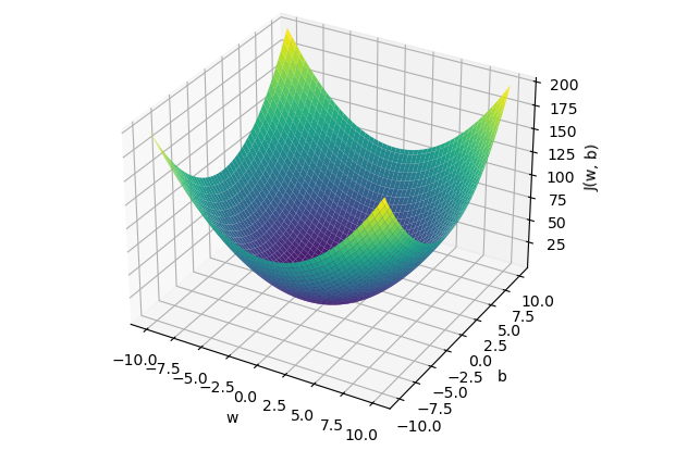
The cost function of linear regression is convex, which means there is a unique set of $w$ and $b$ values that minimize the cost. Let’s visualize three examples to demonstrate this convex shape and the local optimum. For simplicity, we will only consider the cost for $w$, denoted as $J(w)$, in order to represent the cost function in a two-dimensional graph (y-axis $y = J(w)$ and x-axis $x =$ value of $w$). We will test three values of $w$: $w = 0; w = 0.5; w = 1$.

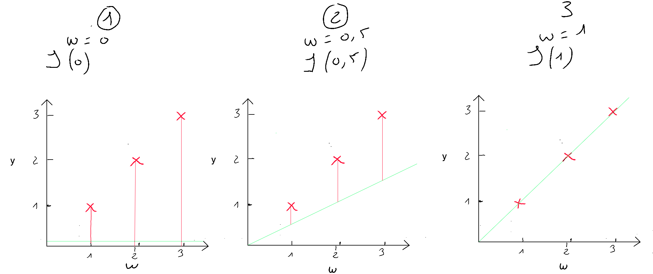
If we apply the simplified cost function to $w$, we get the following $J(w) = \min \frac{1}{2m} \sum_{i=1}^n ((w \cdot x^{(i)}) - y^{(i)})^2$; which we apply to our cases :

1. (1) : $J(0) = \frac{1}{2m} \sum_{i=1}^n (1^2 + 2^2 + 3^2) = \frac{1}{6} (14) = 2.3$ ;
2. (2) : $J(0.5) = \frac{1}{2m} \sum_{i=1}^n ((0.5 - 1)^2 + (1 - 2)^2 + (1.5 - 3)^2) = \frac{1}{6} (3.5) = 0.58$ ;
3. (3) : $J(1) = \frac{1}{2m} \sum_{i=1}^n (wx^{(i)} - y^{(i)})^2 = \frac{1}{2m} \sum_{i=1}^n (0^2 + 0^2 + 0^2) = 0$ ;

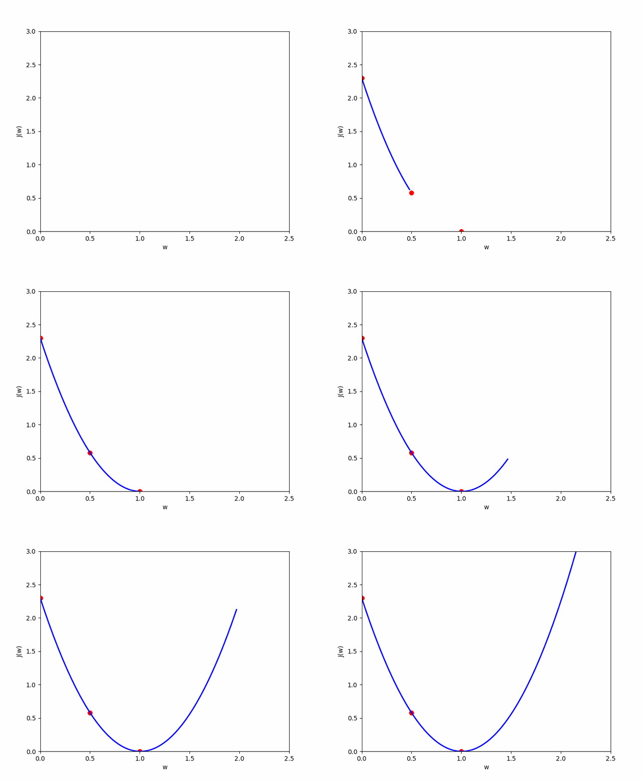
Case number 3 shows us that we have an error of 0. When $w = 1$, the prediction is the best. Now let’s plot these results on a graph where the y-axis represents the cost function result $j(w)$, and the x-axis represents the initialized value of $w$. We can see our three cases ( in green ), and if we test many values for $w$, we will get the other cases ( in yellow ) to eventually discover the convex shape that always ends with a local optimum.

Cost function in Python:

 def compute_cost(x, y, w, b):

    m = x.shape[0]
    cost = 0

    for i in range(m):
        f_wb = w * x[i] + b
        cost = cost + (f_wb - y[i])**2
    total_cost = 1 / (2 * m) * cost
          
    #regularization_cost = (lambda_ / (2 * m)) * np.sum(w**2)
    #total_cost += regularization_cost  
    return total_cost

Gradient Descent

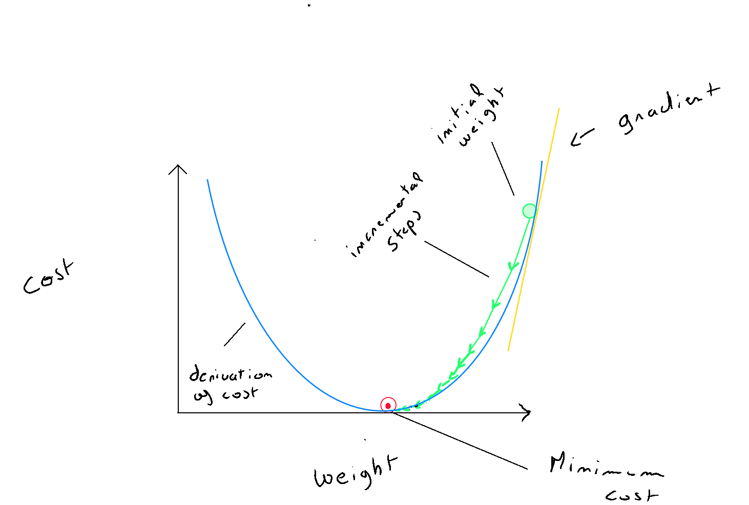
Gradient descent is an optimization algorithm used to find a local minimum of a differentiable function. We have the cost function $J(w, b)$, and the goal of the gradient descent algorithm is to iteratively reduce this cost until reaching $min(J(w, b))$, the local optimum.

Steps

The process is relatively simple :

• Step 1 : Gradient descent starts by applying the cost function : $J(w, b) = \frac{1}{2m} \sum_{i=1}^n ((w \cdot x^{(i)} + b) - y^{(i)})^2$ with random initial values for $w$ and $b$. Based on this calculation, the algorithm finds itself at a certain point on the graphical shape of the cost function (bowl-shaped) ;


• Step 2 : To descend into the trough of the graph and reach the local optimum, at each iteration, the algorithm calculates the derivatives of $w$ $\frac{d}{dw} j(w,b)$ and of $b$ $\frac{d}{db} j(w,b)$, which help determine the slope of the tangent to the graph of the cost function and provide information for parameter updates. The slope indicates the direction to take to reach the local optimum ( e.g. reducing $w$ means moving to the left; increasing $w$ means moving to the right ) ;


• Step 3 : Although the direction is indicated, the data scientist helps the gradient descent algorithm by defining a learning rate, denoted as $α$, which corresponds to the size of the algorithm's « steps » in the identified direction towards the local optimum. This definition is crucial because if alpha is too large, the algorithm may overshoot the local optimum, causing the cost function to increase again. Conversely, if alpha $(α)$ is too small, the algorithm will eventually reach the optimum but will be very slow ;


• Step 4 : The algorithm iterates a certain number of times until the cost function $J(w, b) = \frac{1}{2m} \sum_{i=1}^n ((w \cdot x^{(i)} + b) - y^{(i)})^2$ reduces below a certain threshold, for example $<= 0.001$, meaning the local optimum has been found ;

For code implementation, the values of $w$ and $b$ must be updated at each iteration. However, since the values from the previous iteration are necessary to calculate the derivatives, it is important to temporarily store the new values of $w$ and $b$ before replacing them :

tip

Gradient descent

$J(w, b) = \frac{1}{2m} \sum_{i=1}^n ((w \cdot x^{(i)} + b) - y^{(i)})^2$

1. $temp_w = w - \alpha \frac{d}{dw} J(w, b) = w - \alpha \frac{1}{m} \sum_{i=1}^{m} [f_{w,b}(x^{(i)}) - y^{(i)}] x^{(i)}$ ;
2. $temp_b = b - \alpha \frac{d}{db} J(w, b) = b - \alpha \frac{1}{m} \sum_{i=1}^{m} [f_{w,b}(x^{(i)}) - y^{(i)}]$ ;
3. $w = temp_w$ ;
4. $b = temp_b$ ;

Choosing Iterations and Alpha Value $(α)$

One key point is properly defining the number of iterations and the value of alpha $(α)$, which, combined with the derivatives, determines the « step » size of the algorithm towards the local optimum. Of course, this value depends on the data, and it is crucial not to choose a value that is too small (graph (1)), as learning will be very slow in this case ; nor should the alpha value be too large (graph (3)), as this would cause the gradient descent to miss the local optimum, leading to an increase in the cost function. Graph (2) represents the ideal situation. Regarding the number of iterations, it is recommended to include an « early stop » function so that a large number of iterations can be defined, but if the cost function reduces by less than a certain amount ( e.g. $0.001$ ) between two iterations, the local optimum is considered to be found. It's important to note that even though alpha $(α)$ is fixed, its combination with the derivatives determines both the direction and the step size, and as the algorithm approaches the optimum, these steps will gradually decrease. The choice of lambda depends on the value of alpha. For example, if alpha is set to $0.01$, lambda can be initialized at $1$ or $10$ to achieve a slightly smaller value than $1$ so that the update to $w$ is slightly reduced.

How do you choose alpha $(α)$? The idea is to start with a large alpha ( e.g. 0.3 ). If we notice that the cost increases after an iteration, alpha is too large, and gradient descent misses the local optimum. In this case, we try smaller alpha values like this : ( 0.1, 0.03, 0.01, 0.003, 0.001, etc. ). Below is an example of iterations to find the local optimum on normalized values.

warning

It is important to understand that RMSE ( Root Mean Square Error ) – the evaluation of the model’s predictive ability – is sensitive to: (1) the choice of variables ( in the case of simple linear regression, it is better to have a variable that is highly correlated and explains the variance of the data ), (2) the learning rate, (3) the number of iterations, and (4) the principle of regularization.

Iteration	Cost	dj_dw	dj_db	w	b
0	67.93	6.13	9.98	5.00	10.00
5000	3.39	1.28	2.23	0.35	2.24
10000	0.27	0.27	0.50	-0.62	0.50
15000	0.12	0.06	0.11	-0.82	0.12

Early stopping at iteration 17554 as cost change is less than 0.000001 ( w, b ) found by gradient descent : ( -0.85, 0.06 ).

Gradient descent in Python :

def compute_gradient(x, y, w, b, lambda_):
    m = x.shape[0]
    dj_dw = 0
    dj_db = 0
    for i in range(m):
        f_wb = w * x[i] + b
        dj_dw_i = (f_wb - y[i]) * x[i]
        dj_db_i = f_wb - y[i]
        dj_db += dj_db_i
        dj_dw += dj_dw_i
    dj_dw = dj_dw / m
    dj_db = dj_db / m
    dj_dw += (lambda_ / m) * w
    return dj_dw, dj_db

Launching Gradient Descent :

def gradient_descent(x, y, w_in, b_in, alpha, num_iters, cost_function, gradient_function,lambda_):
    J_history = []
    p_history = []
    b = b_in
    w = w_in

    for i in range(num_iters):
        dj_dw, dj_db = gradient_function(x, y, w , b, lambda_)

       
        b = b - alpha * dj_db
        w = w - alpha * dj_dw

     
        if i<100000:      
            J_history.append( cost_function(x, y, w , b, lambda_))
            p_history.append([w,b])
            
        if i > 1 and abs(J_history[-1] - J_history[-2]) < 0.000001:
            print(f"Early stopping at iteration {i} as cost change is less than 0.000001")
            break 
            
    
        if i% math.ceil(num_iters/100) == 0:
            print(f"Iteration {i:4}: Cost {J_history[-1]} ",
                  f"dj_dw: {dj_dw}, dj_db: {dj_db}  ",
                  f"w: {w}, b:{b}")

    return w, b, J_history, p_history 

lambda_= 0.01
np.set_printoptions(precision=2)
w_init = 5
b_init = 10

iterations = 100000
tmp_alpha = 0.0003

w_final, b_final, J_hist, p_hist = gradient_descent(x_train ,y_train, w_init, b_init, tmp_alpha,
                                                    iterations, compute_cost, compute_gradient, lambda_)

print(f"(w,b) found by gradient descent: ({w_final},{b_final})")

Multiple Predictors

So far, we have covered simple linear regression, where one variable $x$ ( predictor ) explains a variable $\hat{Y}$ ( predicted variable ). Simple linear regression is used to simplify the understanding of the regression model and also because it is useful to visualize the process in two dimensions. However, in reality, we often use a set of columns considered as explanatory variables ( predictors ) for a single predicted variable $\hat{Y}$.

The difference between simple linear regression and multiple linear regression lies in the fact that multiple linear regression uses several $x$: $x_1, x_2, x_3, ..., x_n$. In simple linear regression, gradient descent iterates to find the values of $w$ and $b$, with the formula for simple linear regression being :

$$\hat{Y} = b + w * x$$

In multiple linear regression, we don't have just one line but as many lines as there are $x$ columns. Therefore, each $x$ has its own $w$ parameter. The only element that remains the same, though obviously impacted by all the columns, is the value of $b$, the intercept of the lines.

$$\hat{Y} = b + w_1 x_1^{(i)} + w_2 x_2^{(i)} + w_3 x_3^{(i)} + ... + w_p x_p^{(i)}$$

Each record (i) - each row - will contain a set of values for each column, and consequently, each column will have a « weight » $w$.

Vectorized Computation

In machine learning, vectorized computation is preferred in such cases because vector operations are parallelized, meaning multiple calculations can be performed simultaneously on different elements of the vector. Additionally, GPUs ( Graphics Processing Units ) are very efficient at performing these parallel calculations. Vectors are also stored contiguously in memory ( allowing for faster data access by the processor ). From a human perspective, vector notation simplifies operations, with arrows over $x$ $(\vec{x})$ and $w$ $(\vec{w})$.

The formula :

$$\hat{Y} = b + w_1 x_1^{(i)} + w_2 x_2^{(i)} + w_3 x_3^{(i)} + ... + w_p x_p^{(i)}$$

Can therefore be written as :

$$f_{\vec{w}, b}(\vec{x}) = \vec{w} \cdot \vec{x} + b$$$$\hat{Y} = b + \vec{w} \cdot \vec{x}$$

where
$\vec{x} = [x_1, x_2, x_3, ... , x_n]$
$\vec{w} = [w_1, w_2, w_3, ... , w_n]$

Python Code for Multiple Linear Regression

def predict(x, w, b):
    p = np.dot(x, w) + b
    return p

Polynomial Regression

Up until now, we have discussed linear regression. However, it's important to consider that the distribution of the data might take a non-linear shape, specifically a polynomial one. You may find yourself with a perfectly prepared and trained linear regression model that performs poorly simply because the data distribution is polynomial.

As a data scientist, this is something that cannot be known in advance, which is why the algorithm should include polynomial versions whose evaluations can be compared with the linear form.

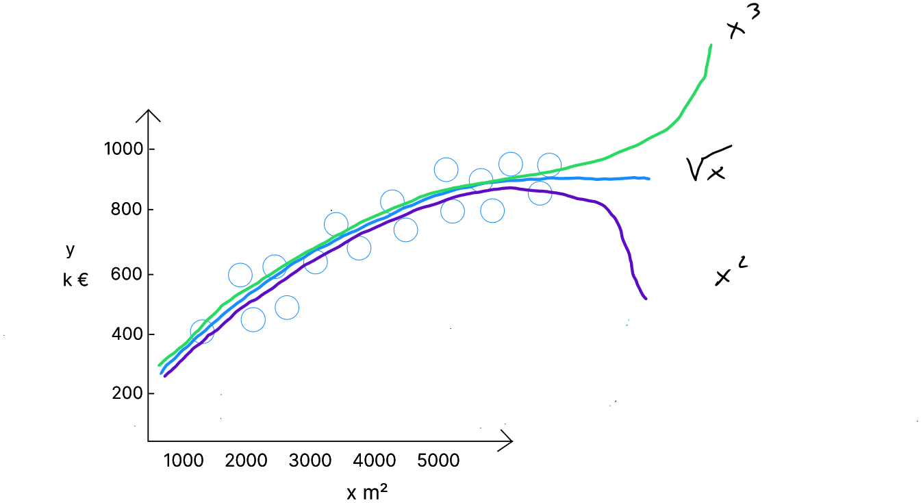
These are curve-shaped ( non-linear ) distributions. In such cases, each variable will be repeated and raised to different powers—up to the degree of the polynomial.

Second-Degree Polynomial Regression

Let's take the example of a second-degree polynomial regression formula.

As a reminder, the linear formula is $\hat{y} = b + w * x$.

If we want to test the second-degree polynomial form ( the purple line in the graph ), we simply duplicate the predictor and square it. This duplicated, squared predictor is considered a separate predictor and will have its own weight.

Thus, for a second-degree polynomial regression, the formula is as follows:

$$\hat{y} = b + w_1 * x + w_2 * x²$$

In the case of a second-degree multiple polynomial regression, each predictor will be repeated and squared.

The coefficient $w_2$ associated with $x²$ controls the curvature of the parabola.

Third-Degree Polynomial Regression

If we want to test the third-degree polynomial form ( the green line in the graph ), we triple the predictor : one version is normal, the other is squared, and the third is cubed. These additional predictors ( squared and cubed ) will be treated as separate predictors, each with its own weight, and their associated weights control the curvature of the parabola.

Composite Regression

There are also « composite » cases, such as a composite regression with a linear term and a square root term ( the blue line in the graph ). In this case, we duplicate each predictor, applying the square root to the duplicate of $x$, which will also have a specific weight.

$$\hat{y} = b + w_1 * x + w_2 * \sqrt{x}$$

warning

Be cautious to avoid overfitting when using high-degree polynomial models, as this might lead to excellent validation scores but poor test performance. Consequently, the model will not generalize well. To prevent overfitting, techniques such as cross-validation, regularization, or limiting the polynomial degree are recommended.

Python Polynomial Function

from sklearn.preprocessing import PolynomialFeatures


x = data[['x_1', 'x_2', 'x_3', 'x_4', 'x_5', '...', 'x_n']].values  
y = data['y'].values  

poly = PolynomialFeatures(degree=3)

scaler_x = StandardScaler()
scaler_y = StandardScaler()

x_poly = poly.fit_transform(x)

y = scaler_y.fit_transform(y.reshape(-1, 1))
x_poly = scaler_x.fit_transform(x_poly)

x_train, x_test, y_train, y_test = train_test_split(x_poly, y, test_size=0.4, random_state=42)

Regularization

As discussed in the section on supervised learning, we may encounter situations of either underfitting or overfitting.

To recap, in underfitting, the validation stage ( i.e. applying the model to the data it was trained on ) will yield poor results. The model is not rich enough to create a generalizable rule. Underfitting is less common, and the main option for a data scientist is to acquire more variables or records that will help the model better identify relationships.

In overfitting, there are several techniques to prevent the model - which performs very well on the training data - from failing to establish a generalizable rule.

The first option is similar to underfitting : the model may not have enough records for the number of variables used, leading it to « fit » too closely to the training data.

The second option involves increasing or reducing the number of variables ( Variable Selection ). Increasing the number of variables can ensure better data dispersion, helping the model establish a more generalizable rule. However, it is more common for the model to use too many variables, and the goal is to reduce the number of variables through feature engineering.

To reduce the number of variables, there are specific techniques, but sometimes keeping all the variables is necessary. Regularization can help in such cases by mitigating overfitting.

Consider the following equation :

$$\hat{Y} = b + w_1 x_1^{(i)} + w_2 x_2^{(i)} + w_3 x_3^{(i)} + ... + w_p x_p^{(i)}$$

If, for some reason, the gradient descent optimization assigns the weight $w_3$ of variable $x_3$ to $0$, the values of $x_3$ would be nullified by the model's weight, effectively removing that variable from the model.

Regularization reduces the impact of certain variables by assigning them smaller weights. Specifically, the idea is for the learning algorithm to reduce parameter values without requiring any to be zero. This reduction in some parameters helps optimize the model's regularization, preventing it from overfitting the training data. Regularization mainly applies to the $w$ values, though it can also affect the $b$ parameter.

The regularization function can be applied by modifying the cost function. The idea is to achieve smaller parameter values for $w$ to simplify the model. The challenge lies in distinguishing which variables should be penalized - those contributing to overfitting - from those that should be kept. In regularization, all variables are penalized.

This penalty is applied by adding regularization to the cost function :

$$J(w, b) = \min \frac{1}{2m} \sum_{i=1}^n (f(w,b)x^{(i)} - y^{(i)})^2 \textcolor{blue}{+ \frac{\lambda}{2m} \sum_{j=1}^n w_j^2}$$

It's also possible to apply regularization to the $b$ parameter :

$$J(w, b) = \min \frac{1}{2m} \sum_{i=1}^n (f(w,b)x^{(i)} - y^{(i)})^2 \textcolor{blue}{+ \frac{\lambda}{2m} \sum_{j=1}^n w_j^2} + \textcolor{red}{\frac{\lambda}{2m}b^2}$$

$\lambda$ is the regularization parameter, and like we did previously with the learning rate $(\alpha)$ for the gradient descent algorithm, it's up to us, as data scientists, to define its value. Dividing $\lambda$ by $2*m$ serves to normalize the regularization with the rest of the function, making it easier to choose the value for $\lambda$.

tip

Regularized Gradient Descent ( w only )

$J(w, b) = \frac{1}{2m} \sum_{i=1}^n ((w \cdot x^{(i)} + b) - y^{(i)})^2 \textcolor{blue}{+ \frac{\lambda}{2m} \sum_{j=1}^n w_j^2}$

1. $temp_w = w - \alpha \frac{d}{dw} J(w, b) = w - \alpha \left( \frac{1}{m} \sum_{i=1}^{m} [f_{w,b}(x^{(i)}) - y^{(i)}] x^{(i)} + \textcolor{blue}{\frac{\lambda}{m} w_j}\right)$ ;
2. $temp_b = b - \alpha \frac{d}{db} J(w, b) = b - \alpha \left(\frac{1}{m} \sum_{i=1}^{m} [f_{w,b}(x^{(i)}) - y^{(i)}]\right)$ ;
3. $w = temp_w$ ;
4. $b = temp_b$ ;

Full Python Code

import numpy as np
import pandas as pd
from sklearn.preprocessing import StandardScaler
from sklearn.model_selection import train_test_split
import math, copy
from sklearn.metrics import mean_squared_error
from sklearn.preprocessing import PolynomialFeatures

data = pd.read_csv('data.csv')
data

x = data[['x_1', 'x_2', 'x_3', 'x_4', 'x_5', '...', 'x_n']].values  
y = data['y'].values  


scaler_x = StandardScaler()
scaler_y = StandardScaler()

x = scaler_x.fit_transform(x)
y = scaler_y.fit_transform(y.reshape(-1, 1))

x_train, x_test, y_train, y_test = train_test_split(x, y, test_size=0.4, random_state=42)

#Polynomial 
"""
x = data[['x_1', 'x_2', 'x_3', 'x_4', 'x_5', '...', 'x_n']].values  
y = data['y'].values  

poly = PolynomialFeatures(degree=3)

scaler_x = StandardScaler()
scaler_y = StandardScaler()

x_poly = poly.fit_transform(x)

y = scaler_y.fit_transform(y.reshape(-1, 1))
x_poly = scaler_x.fit_transform(x_poly)

x_train, x_test, y_train, y_test = train_test_split(x_poly, y, test_size=0.4, random_state=42)
"""
#/Polynomial 

def predict(x, w, b):
    p = np.dot(x, w) + b
    return p

def compute_cost(X, y, w, b):
    m = X.shape[0]
    cost = 0.0
    for i in range(m):
        f_wb_i = np.dot(X[i], w) + b           
        cost = cost + (f_wb_i - y[i])**2       
    cost = cost / (2 * m)

    # regularisation L2 (ridge)
    regularization_cost = (lambda_ / (2 * m)) * np.sum(w**2)
    cost += regularization_cost                    
    return cost

def compute_gradient(X, y, w, b,lambda_):
    m,n = X.shape           
    dj_dw = np.zeros((n,))
    dj_db = 0.

    for i in range(m):
        err = (np.dot(X[i], w) + b) - y[i]
        for j in range(n):
            dj_dw[j] = dj_dw[j] + err * X[i, j]
        dj_db = dj_db + err
    dj_dw = dj_dw / m
    dj_db = dj_db / m
    dj_dw += (lambda_ / m) * w

    return dj_db, dj_dw

def gradient_descent(X, y, w_in, b_in, cost_function, gradient_function, alpha, num_iters, lambda_):
    J_history = []
    w = copy.deepcopy(w_in)  
    b = b_in

    for i in range(num_iters):
        dj_db,dj_dw = gradient_function(X, y, w, b, lambda_)  
        w = w - alpha * dj_dw               
        b = b - alpha * dj_db               

        if i<100000:      
            J_history.append( cost_function(X, y, w, b, lambda_))
        
        if i > 1 and abs(J_history[-1] - J_history[-2]) < 0.000001:
            print(f"Early stopping at iteration {i} as cost change is less than 0.000001")
            break 
            
        if i% math.ceil(num_iters / 10) == 0:
            print(f"Iteration {i:4}: Cost {J_history[-1]} ",
                  f"dj_dw: {dj_dw}, dj_db: {dj_db}  ",
                  f"w: {w}, b:{b}")

    return w, b, J_history 

initial_w = np.random.randn(7) 
initial_b =  0    

lambda_ = 0.01
iterations = 10000
alpha = 0.0001 
w_final, b_final, J_hist = gradient_descent(x_train, y_train, initial_w, initial_b,
                                                    compute_cost, compute_gradient,
                                                    alpha, iterations, lambda_)

print(f"(w,b) found by gradient descent: ({w_final},{b_final})")

Model Evaluation

For model evaluation, we use the RMSE - Root Mean Square Error - evaluation of an estimation model.

def predict(X, w, b):

    return np.dot(X, w) + b 


def rmse(y_true, y_pred):
    mse = np.mean((y_true - y_pred) ** 2)
    return np.sqrt(mse)

y_pred = predict(x_test, w_final, b_final)

y_pred_original = scaler_y.inverse_transform(y_pred.reshape(-1, 1))
y_test_original = scaler_y.inverse_transform(y_test.reshape(-1, 1))

rmse_value_original = rmse(y_test_original, y_pred_original)

rmse_percentage = (rmse_value_original / np.mean(y_test_original)) * 100

print(f"RMSE on the test set (original scale): {rmse_value_original}")
print(f"RMSE en pourcentage sur l'ensemble de test: {rmse_percentage:.2f}%")

Prediction Based on New $x$ Values

x_new = np.array([[value_1, value_2, value_3, value_4, value_5, ..., value_n]]) 
x_new_normalized = scaler_x.transform(x_new)
y_new_normalized = np.dot(x_new_normalized, w_final) + b_final
y_new_normalized = y_new_normalized.reshape(-1, 1) 
y_new = scaler_y.inverse_transform(y_new_normalized)
print(f"Predicted value : {y_new[0][0]}")

Polynomial
"""
x_new = np.array([[value_1, value_2, value_3, value_4, value_5, ..., value_n]]) 
x_new_poly = poly.transform(x_new)  # Transformer les nouvelles données pour inclure les termes polynomiaux
x_new_normalized = scaler_x.transform(x_new_poly)
y_new_normalized = np.dot(x_new_normalized, w_final) + b_final
y_new_normalized = y_new_normalized.reshape(-1, 1)
y_new = scaler_y.inverse_transform(y_new_normalized)

print(f"Predicted value : {y_new[0][0]}") 
"""