Decision Tree
The decision tree is one of the most powerful techniques in supervised learning and could be placed at the same level as neural networks if these two techniques were part of the same family.
So far, we have covered so-called « parametric » techniques, meaning techniques where the goal of learning is to identify parameters explaining a relationship between explanatory variables ( predictors ) and an explained ( or predicted ) variable, . Identifying these parameters is achieved through a series of iterations aimed at minimizing a cost function.
The decision tree is a non-parametric technique, meaning there are no parameters explaining the relationship between and . It is one of the most used techniques because it is easily understandable ( interpretable ) and can handle missing data.
The tree technique in which the target variable is qualitative is called a « classification tree », and the one where the target variable contains quantitative values is called a « regression tree. »
Applying a decision tree model involves starting with the entire dataset and recursively splitting it into smaller and smaller cells that become increasingly pure in the sense that they have similar values to the target. The data is split into segments based on splitting rules at each stage. Taken together, the rules of all segments form the decision tree model.
A decision tree is, therefore, a hierarchical set of rules that describe successive divisions of a large dataset into groups of smaller records. With each successive division, the members of the resulting segments become more and more alike until they can be assimilated to the target variable.
To benefit from an accurate decision tree model, the algorithm must rely on a significant number of records. However, unlike other techniques, once the trees are built, the calculations are not performance-intensive. Moreover, the decision tree is a highly automated technique, resistant to outliers, and capable of handling missing values.
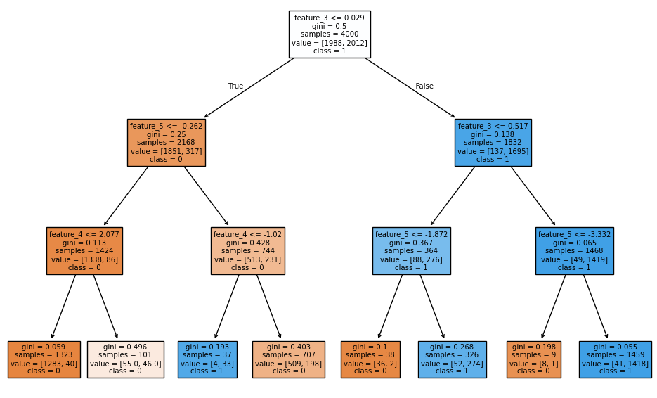
One of the reasons decision trees are so popular is that they provide easily understandable decision rules. IF Age ≤ 55 AND Education > 12 THEN Class = 1 ELSE ; Each subgroup resulting from the division contains a set of homogeneous records.
Some of the diagrams and concepts presented here are inspired by the Machine Learning course by Andrew Ng, a program created in collaboration between Stanford University Online Education and DeepLearning.AI, available on Coursera. Find the original course here: Machine Learning by Andrew Ng.
Structure
A decision tree always starts at the root node, which contains all the records. The tree will test all the variables in the root node to identify the variable that best splits the data. The data is then distributed into two decision nodes, which, in turn, will test all the variables to identify the best information split into « purer information. » These divisions are repeated, and at each step, the information either lands in a new decision node ( new division of the records ) or in a terminal node where the information is considered to have reached a certain purity.
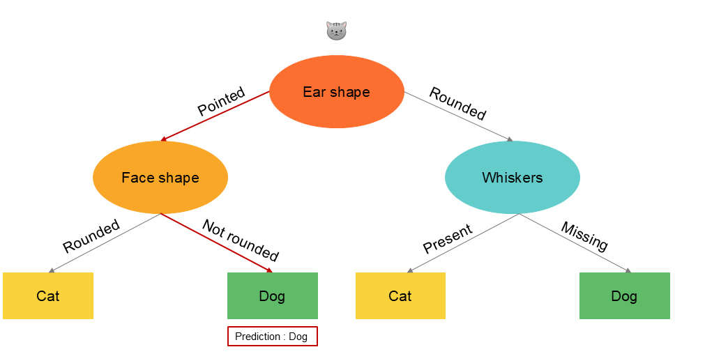
Let's take the following example to illustrate a decision tree. We'll start with a classification tree. We have data on cats and dogs, and we want to train a decision tree algorithm to predict whether a new animal is a dog or a cat based on its characteristics. Our dataset contains three qualitative variables ( which should normally be transformed into one-hot encoding ) and a variable representing a value of for a cat and for a dog.

| Ear Shape x1 | Face Shape x2 | Whiskers x3 | Cat y |
|---|---|---|---|
| Pointed | Rounded | Present | 1 |
| Floppy | Not rounded | Present | 1 |
| Floppy | Rounded | Absent | 0 |
| Pointed | Not rounded | Present | 0 |
| Pointed | Rounded | Present | 1 |
| Pointed | Rounded | Absent | 1 |
| Floppy | Not rounded | Absent | 0 |
| Pointed | Rounded | Absent | 1 |
| Floppy | Rounded | Absent | 0 |
| Floppy | Rounded | Absent | 0 |
For a new record, we want a model that allows us to identify whether it is a dog or a cat.
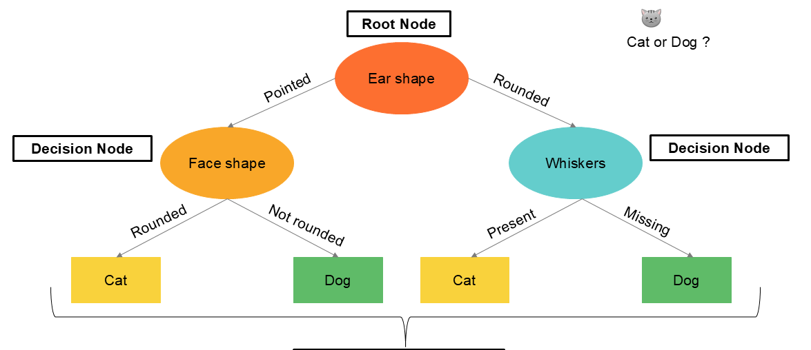
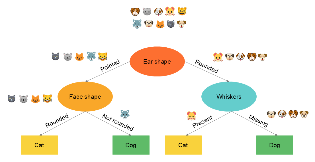
Here is an example of a trained model in our case :
Recursive Partitioning
The key concept in building a tree is the recursive partitioning of information. This involves grouping records by dividing them into subpopulations based on a splitting value. This division is done recursively, meaning that it operates on the results of the previous division.
Recursion means constructing a decision tree at the root by building smaller decision trees in the left and right sub-branches. All variables are considered at each step to identify which one will best split the information, i.e. lead to purer nodes after the split.
In computing, recursion involves writing code that calls itself. When constructing a decision tree, we build the overall decision tree by constructing smaller decision sub-trees and then assembling them. That’s why software implementations of decision trees sometimes refer to a recursive algorithm.
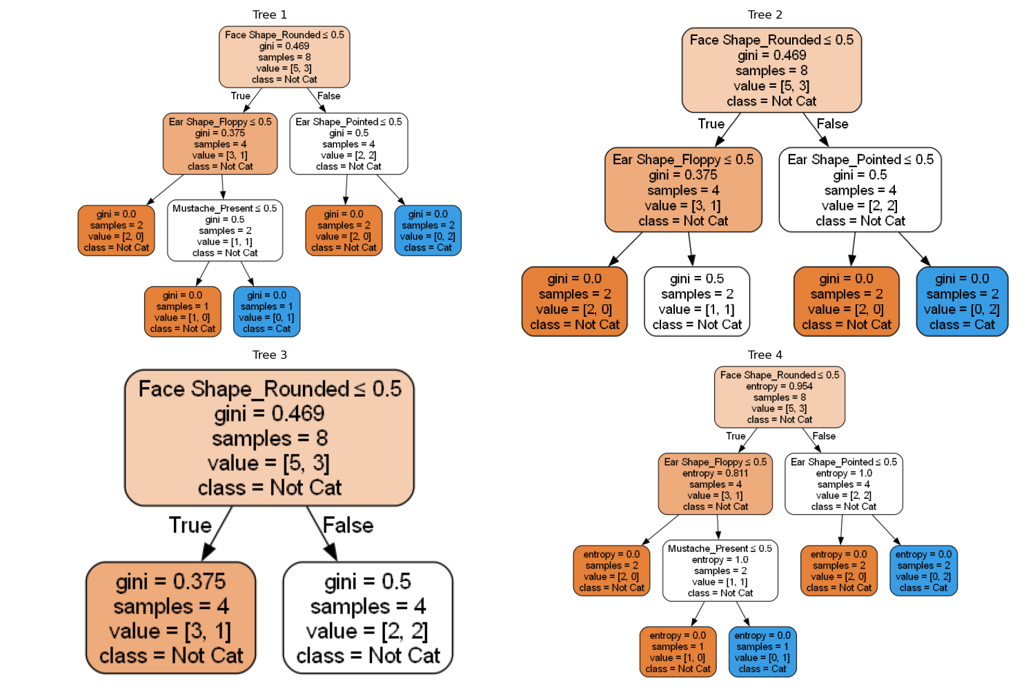
This partitioning is defined by an arbitrary choice of the data scientist on the tree's depth. The greater the maximum depth, the larger the decision tree, allowing it to learn a more complex model while also increasing the risk of overfitting.
Therefore, there are different ways to create a decision tree. Here are some examples of alternatives in our illustrated case. Among these versions, some will perform better than our base tree, while others will perform worse when we evaluate the model on the test data. We will select the one that performs best but also has a generalizable rule.
Learning Process
The steps of the decision tree can be summarized as follows :
We designate the target variable ( output ) and the input variables ( predictors ) . Predictors can be quantitative or qualitative, but in the latter case, they must be transformed using the one-hot encoding technique for nominal qualitative variables or digitisation for ordinal qualitative variables.
- Step 1 : we start with all records in the root node ;
- Step 2 : calculate the information gain for all 𝑋_𝑖 and select the variable with the highest gain ;
- Step 3 : for this variable 𝑋_𝑖, split the records into a left branch ( left decision node ) or a right branch ( right decision node ) ;
- Step 4 : repeat the process until a stopping criterion is met ;
The first decision the algorithm makes is to determine which variable will be considered in the root node to create the first data split. Then, what variables will be considered in the subdivisions of subsequent nodes down to the terminal leaves.
The choice of the input variable for splitting the root node is crucial as it enables the first data split into subgroups containing more homogeneous values. The question is, therefore, how to choose the best node and what are the best child nodes of a parent node. The goal is to separate the target values as much as possible. The algorithm will consider all possible splits across all input variables based on the best split value.
The algorithm's objective is to identify the first variable that maximizes purity or minimizes impurity.
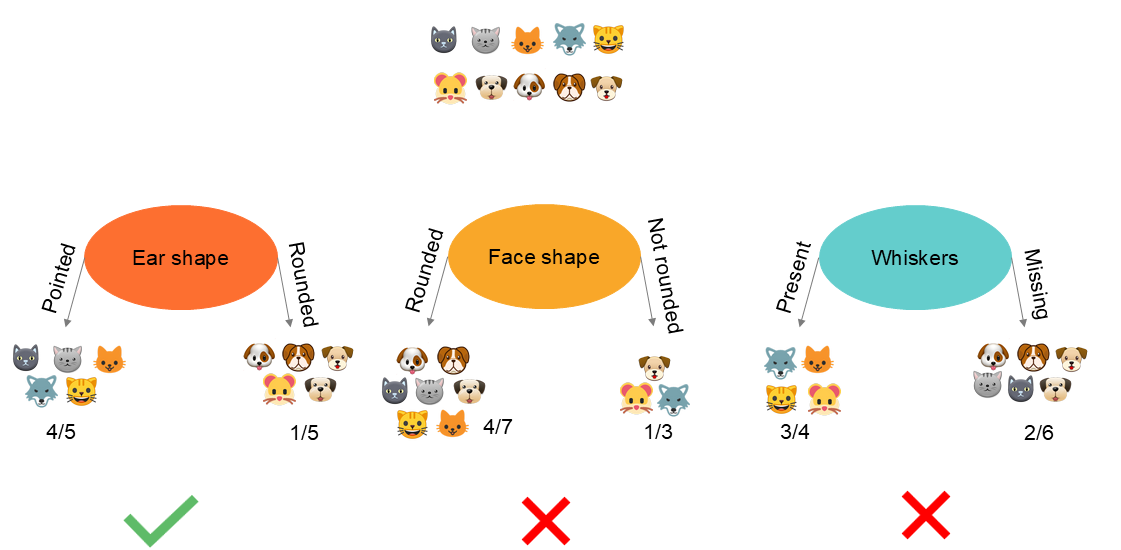
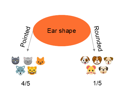
In the example above, we see that partitioning the information based on ear shape leads to a purer split, i.e. achieving the best separation between cats and dogs. This example is relatively simple because we visualize the result. Of course, there are indicators.
Impurity Measure
The goal of a tree is to achieve « purer » nodes after splitting the information. Impurity is an index that helps us identify the resulting node that contains the most homogeneous values. Impurity is measured by Entropy.
Probability :
Entropy :
Let’s begin by calculating entropy, i.e. the measure of impurity. The principle is as follows : the more a node contains similar values, the purer it is.
Let’s take the following example of four predictors ( ear shape , face shape , presence of whiskers ) that were used to split the information. In the first case, the resulting node contains 2 cats and 4 dogs. corresponds to . In the second case, the node contains 3 cats and 3 dogs. corresponds to . We know for each case, and we need to calculate the entropy formula knowing that . We obtain the following values :
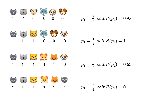
Entropy calculation details for each case :
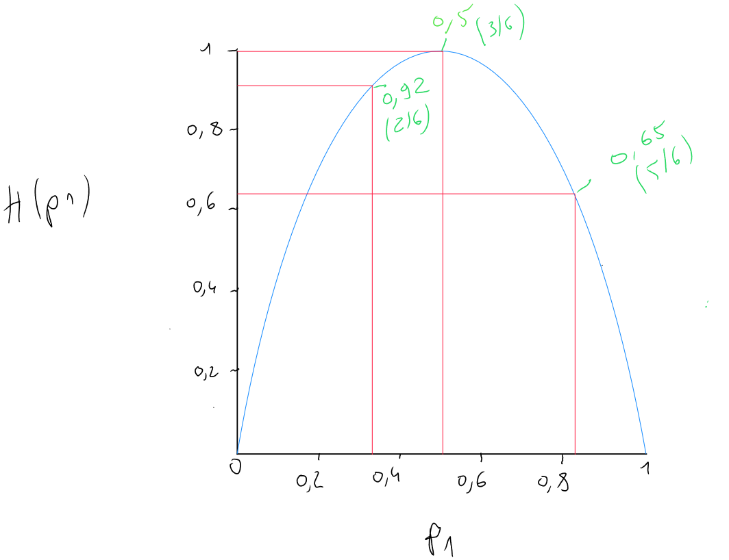
We see that when we obtain a group containing half cats and half dogs, entropy equals 1. Entropy is at its maximum, meaning we are in complete impurity. The node is heterogeneous ( we want a homogeneous node containing only dogs or cats ). Conversely, when we obtain a completely homogeneous node ( only cats ), we observe that entropy equals , indicating complete purity.
We can graphically represent these examples by plotting probability on the x-axis and entropy on the y-axis to see the impact of probability and the various cases.
Information Gain
Entropy allows us to calculate impurity, but what interests us is identifying the variable that will help reduce this impurity. The reduction in entropy is called « information gain ». Information gain corresponds to the result of moving from state to state , in other words, from the root node, where all the records are found, to the next node. Let’s imagine that we have 5 cats and 5 dogs, so we have an entropy of 1 corresponding to the function (5 cats / 5 dogs, so and ).
We start from a value of at the root node, and we calculate the result of subtracting the entropy of the two resulting nodes after using a variable as a splitter.
Case 1
Information Gain
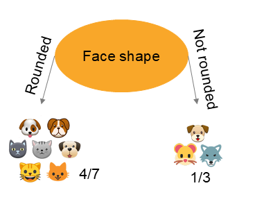
Case 2
Information Gain
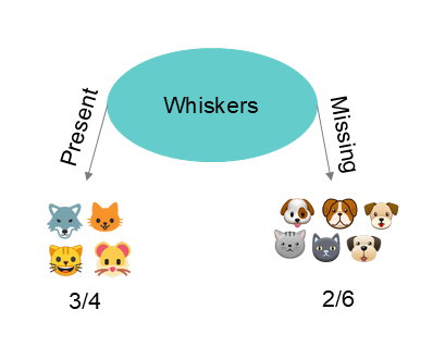
Case 3
Information Gain
Case achieves an information gain of after splitting the records based on the ear shape variable into two new nodes. This is, therefore, the best splitting variable. The operation will then repeat for each subsequent subdivision.
Information gain is calculated as follows :
- (1) Entropy value of the starting node ( before splitting into left and right nodes ) ;
- (2) Number of values in the final left decision node / total number of values in the starting node ;
- (3) Entropy of the number of values in the final left decision node / total number of values in the left decision node ;
- (4) Number of values in the final right decision node / total number of values in the starting node ;
- (5) Entropy of the number of values in the final right decision node / total number of values in the right decision node ;
Example :
Tree Depth
The tree algorithm will divide each node into new lower nodes ( left and right ), with the information becoming purer with each division. One fundamental question in tree creation ( the second most important question after defining purity ) is how deep the algorithm should go, i.e. when it should stop creating subdivisions.
- When a node contains of the same class ( classification ) ; when the variance of a node is less than or equal to a certain threshold ( regression ) ;
- When the split of a node exceeds the maximum desired depth ;
- When the improvement in purity score is below a threshold ;
- When the number of examples in a node is below a threshold ;
Qualitative Predictors
Qualitative variables must be converted into a numerical representation before being used in the tree-building process as predictors.
If the variables are of ordinal qualitative type, they must be digitised. If the variables are of nominal qualitative type, we must apply one-hot encoding.
Quantitative Predictor
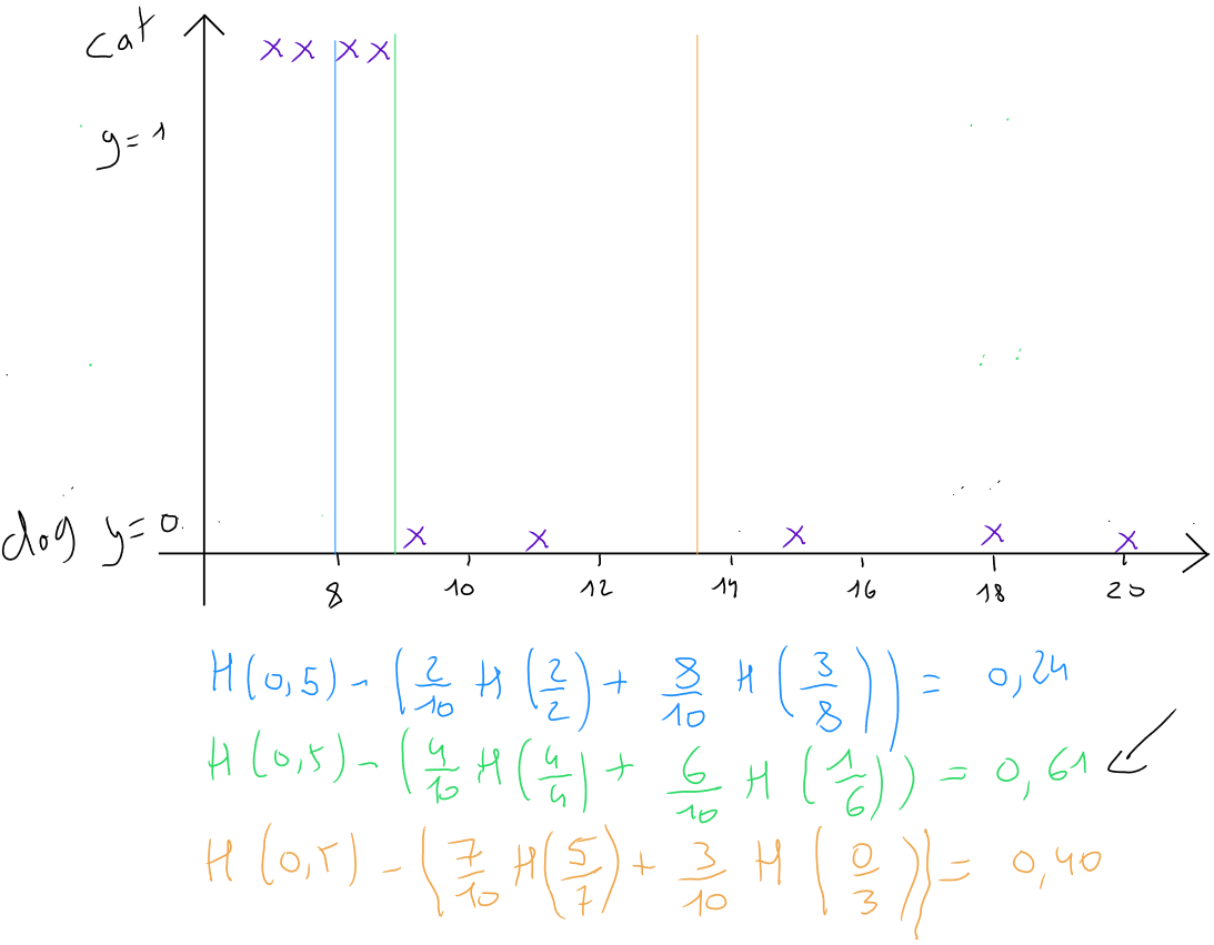
When we have quantitative predictors, the decision tree algorithm works similarly in terms of splitting the information, meaning it analyzes the best data split for the best information gain. However, since there are no classes, the algorithm will use the median value of each pair of consecutive values in the dataset and select the one that provides the best information gain.
Let’s take the example of a new predictor in our dataset for our classification tree, namely weight.
| Ear Shape x1 | Face Shape x2 | Whiskers x3 | Weight x4 | Cat y |
|---|---|---|---|---|
| Pointed | Rounded | Present | 7.2 | 1 |
| Floppy | Not rounded | Present | 8.8 | 1 |
| Floppy | Rounded | Absent | 15 | 0 |
| Pointed | Not rounded | Present | 9.2 | 0 |
| Pointed | Rounded | Present | 8.4 | 1 |
| Pointed | Rounded | Absent | 7.6 | 1 |
| Floppy | Not rounded | Absent | 11 | 0 |
| Pointed | Rounded | Absent | 10.2 | 1 |
| Floppy | Rounded | Absent | 18 | 0 |
| Floppy | Rounded | Absent | 20 | 0 |
Data must be sorted in ascending order based on the quantitative variable.
Regression Tree
When the target variable - the variable to predict - is quantitative, we apply the regression tree technique. Let’s take the following example: we want to predict the weight of dogs and cats based on the predictors.
| Ear Shape x1 | Face Shape x2 | Whiskers x3 | Weight y |
|---|---|---|---|
| Floppy | Not rounded | Present | 8.8 |
| Floppy | Rounded | Absent | 15 |
| Pointed | Not rounded | Present | 9.2 |
| Pointed | Rounded | Present | 8.4 |
| Pointed | Rounded | Absent | 7.6 |
| Floppy | Not rounded | Absent | 11 |
| Pointed | Rounded | Absent | 10.2 |
| Floppy | Rounded | Absent | 18 |
| Floppy | Rounded | Absent | 20 |
To choose the best node splits - meaning the variable that allows a purer division - the regression tree does not use entropy ( which is only useful for classification ) but selects the division that best reduces within-group variance.
Remember, variance is a measure of the dispersion of values in a variable. It is the average of the squared differences from the mean, is always positive, and is written as follows :
.
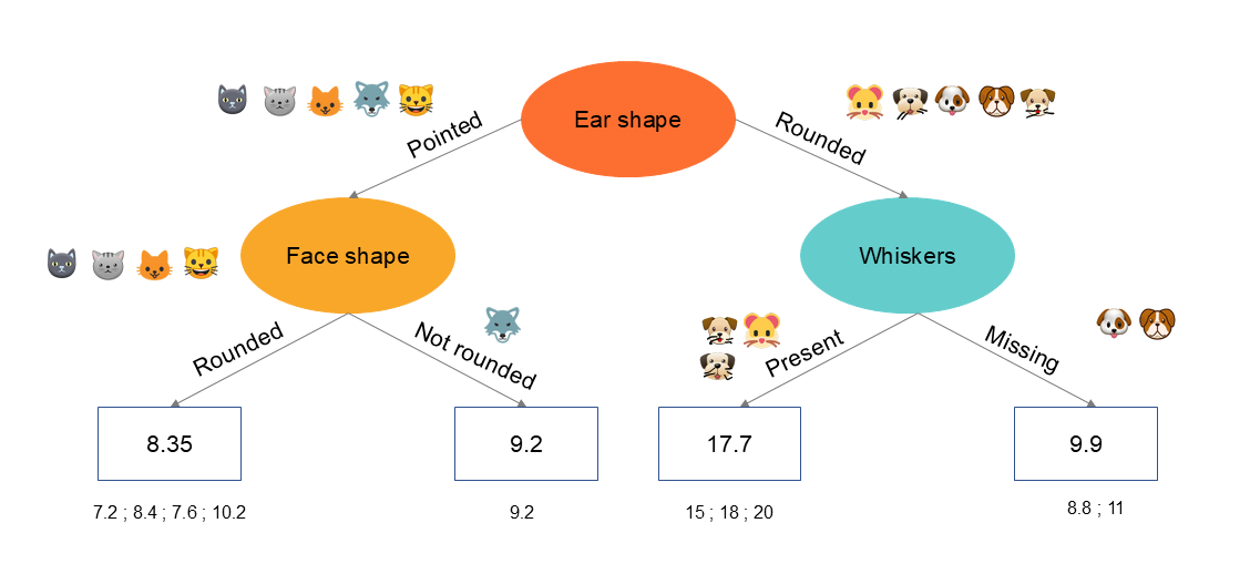
In the example below, the root node contains all the records and has a variance of . The algorithm will test all the predictors to identify the one that best splits the information into two decision nodes, reducing the variance the most.
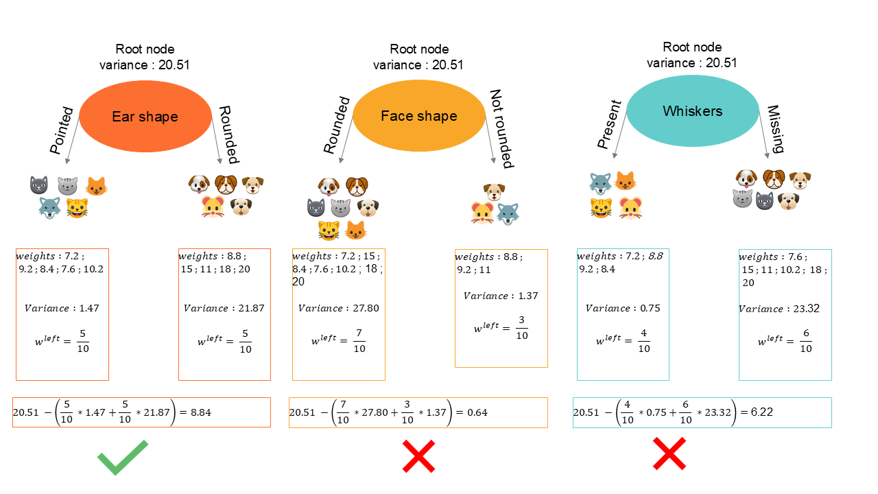
The regression tree algorithm will split each node into new lower nodes ( left and right ) based on variance reduction. The subdivision continues until a stopping criterion is met :
- When the variance of a node is less than or equal to a certain threshold ( regression ) ;
- When the split of a node exceeds the maximum desired depth ;
- When the number of examples in a node is below a threshold ;
The final value of a new record will be predicted based on the average of the values in that node :
Ensemble of Trees
One of the weaknesses of using a single decision tree is that it can be very sensitive to small changes in the data.
Adding new data can significantly change the tree's structure, meaning the algorithm's selection of discriminating variables. Changing one data point in the training set can lead to the characteristic with the highest information gain becoming, for example, the presence of whiskers instead of ear shape. As a result, the subsets of data obtained in the left and right sub-trees become completely different.
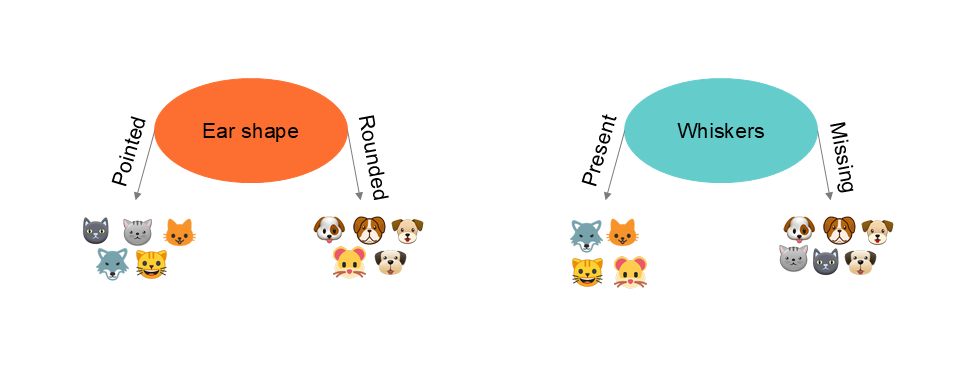
A more robust solution to avoid this problem is to construct not just one decision tree but a large number of decision trees, which we call an ensemble of trees.
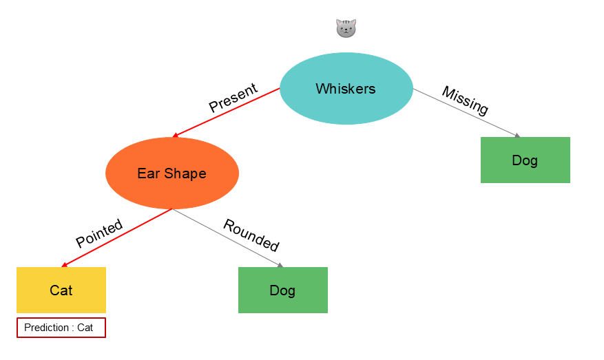
Let’s take the case of predicting a new record in the dataset and see three cases of trees fed with different data :
| Ear Shape x1 | Face Shape x2 | Whiskers x3 | Cat y |
|---|---|---|---|
| Pointed | Not rounded | Present | ? |
Random Forest
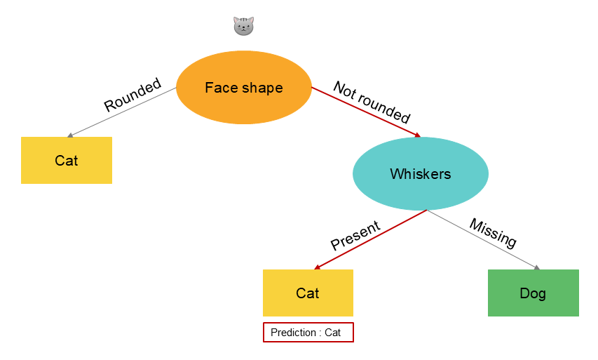
The concept of Random Forests is to generate several tree structures based on random subsets of the training data. We use multiple trees, which lead to different predictions, and we consider the majority prediction as the final prediction. By having many decision trees and having them vote, the overall algorithm becomes less sensitive and more robust.
In the example below, we use three trees, which lead to different predictions, but the majority identifies the record as a cat.
As data scientists, the question we must ask is how to find all these possible decision trees.
We apply a method of random sampling, in which elements are selected at random from the dataset. The resulting subset is used to «train» a first decision tree. Then, each selected record is returned to the dataset before another random subset is selected to train a second decision tree, and so on.
By applying this method, each random sample can be different, allowing for the creation of multiple distinct trees. This process reduces variance and improves the predictive performance of the trees, avoiding overfitting. By combining the predictions of multiple trees, we obtain more robust and accurate predictions.
Random Forest is a supervised learning algorithm that combines multiple decision trees to improve predictive performance. To build a Random Forest model, several decision trees are constructed from random samples created from the original dataset using sampling with replacement.
Each decision tree is trained on a different random sample and uses a random subset of the available features to construct the tree :
Random Forest is a popular algorithm due to its robustness, ability to handle missing data or outliers, and capability to manage large datasets with numerous features.
Steps :
- ;
- Use random subsampling to create a new training dataset of size and build a new decision tree ;
- B, according to the literature, takes a value between 64 and 228. Generally, we don’t exceed 1000 as it has been shown that more than 1000 trees don’t bring significant improvement and instead slow down computations ;
- Each decision tree is used to make a prediction, and the final prediction is the average ( for a continuous variable ) or the mode ( for a categorical variable ) of the predictions from all the decision trees ;
Xboost
The Xboost algorithm is also a random forest algorithm. It operates similarly to the random forest algorithm : several decision trees are constructed from random samples created from the original dataset. Then, each selected record is returned to the dataset before another subset is selected to train a second decision tree.
Unlike Random Forest, which takes a completely random subset of data, the Xboost algorithm favors the probability of selecting records already used by previous trees and whose predictions were incorrect.
Steps :
- ;
- Use random subsampling to create a new training dataset of size and build a new decision tree. Instead of purely random selection, Xboost favors selecting data examples that were not correctly predicted by the previously trained trees ;
- B, according to the literature, takes a value between 64 and 228. Generally, we don’t exceed 100 as it has been shown that more than 100 trees don’t bring significant improvement and instead slow down computations ;
- Each decision tree is used to make a prediction, and the final prediction is the average ( for a continuous variable ) or the mode ( for a categorical variable ) of the predictions from all the decision trees ;
Python Code
Decision Tree
pip install xgboost
import numpy as np
import pandas as pd
from sklearn.tree import DecisionTreeClassifier
from sklearn.ensemble import RandomForestClassifier
from sklearn.model_selection import train_test_split
from sklearn.metrics import accuracy_score
from xgboost import XGBClassifier
import matplotlib.pyplot as plt
RANDOM_STATE = 55


data = pd.read_csv("data.csv")
cat_variables = ['Column_1','Column_2','Column_3','Column_4','Column_5']

df = pd.get_dummies(data = df,prefix = cat_variables,columns = cat_variables)

features = [x for x in df.columns if x not in 'NameColumnY']

X_train, X_val, y_train, y_val = train_test_split(df[features], df['NameColumnY'], train_size = 0.8, random_state = RANDOM_STATE)


min_samples_split_list = [2,10, 30, 50, 100, 200, 300, 700] ,
max_depth_list = [1,2, 3, 4,5,6, 8, 16, 32, 64, None] # None = no depth limit.
Identification of min_samples_split
accuracy_list_train = []
accuracy_list_val = []
for min_samples_split in min_samples_split_list:
    # You can fit the model at the same time you define it, because the fit function returns the fitted estimator.
    model = DecisionTreeClassifier(min_samples_split = min_samples_split,
                                   random_state = RANDOM_STATE).fit(X_train,y_train)
    predictions_train = model.predict(X_train) ## The predicted values for the train dataset
    predictions_val = model.predict(X_val) ## The predicted values for the test dataset
    accuracy_train = accuracy_score(predictions_train,y_train)
    accuracy_val = accuracy_score(predictions_val,y_val)
    accuracy_list_train.append(accuracy_train)
    accuracy_list_val.append(accuracy_val)

plt.title('Train x Validation metrics')
plt.xlabel('min_samples_split')
plt.ylabel('accuracy')
plt.xticks(ticks = range(len(min_samples_split_list )),labels=min_samples_split_list)
plt.plot(accuracy_list_train)
plt.plot(accuracy_list_val)
plt.legend(['Train','Validation'])
Identification of max_depth
accuracy_list_train = []
accuracy_list_val = []
for max_depth in max_depth_list:
    model = DecisionTreeClassifier(max_depth = max_depth,
                                   random_state = RANDOM_STATE).fit(X_train,y_train)
    predictions_train = model.predict(X_train)
    predictions_val = model.predict(X_val)
    accuracy_train = accuracy_score(predictions_train,y_train)
    accuracy_val = accuracy_score(predictions_val,y_val)
    accuracy_list_train.append(accuracy_train)
    accuracy_list_val.append(accuracy_val)

plt.title('Train x Validation metrics')
plt.xlabel('max_depth')
plt.ylabel('accuracy')
plt.xticks(ticks = range(len(max_depth_list )),labels=max_depth_list)
plt.plot(accuracy_list_train)
plt.plot(accuracy_list_val)
plt.legend(['Train','Validation'])
Run and adapt parameters
decision_tree_model = DecisionTreeClassifier(min_samples_split = 50, #Change based on chart result
                                             max_depth = 4, #Change based on chart result
                                             random_state = RANDOM_STATE).fit(X_train,y_train)
print(f"Metrics train:\n\tAccuracy score: {accuracy_score(decision_tree_model.predict(X_train),y_train):.4f}")
print(f"Metrics validation:\n\tAccuracy score: {accuracy_score(decision_tree_model.predict(X_val),y_val):.4f}")
Random Forest
pip install xgboost
import numpy as np
import pandas as pd
from sklearn.tree import DecisionTreeClassifier
from sklearn.ensemble import RandomForestClassifier
from sklearn.model_selection import train_test_split
from sklearn.metrics import accuracy_score
from xgboost import XGBClassifier
import matplotlib.pyplot as plt
RANDOM_STATE = 55


data = pd.read_csv("data.csv")
cat_variables = ['Column_1','Column_2','Column_3','Column_4','Column_5']

df = pd.get_dummies(data = df,prefix = cat_variables,columns = cat_variables)

features = [x for x in df.columns if x not in 'NameColumnY']

X_train, X_val, y_train, y_val = train_test_split(df[features], df['NameColumnY'], train_size = 0.8, random_state = RANDOM_STATE)

min_samples_split_list = [2,10, 30, 50, 100, 200, 300, 700]
max_depth_list = [2, 4, 8, 16, 32, 64, None]
n_estimators_list = [10,50,100,500]
Identification of min_samples_split
accuracy_list_train = []
accuracy_list_val = []
for min_samples_split in min_samples_split_list:
    model = RandomForestClassifier(min_samples_split = min_samples_split,
                                   random_state = RANDOM_STATE).fit(X_train,y_train)
    predictions_train = model.predict(X_train)
    predictions_val = model.predict(X_val)
    accuracy_train = accuracy_score(predictions_train,y_train)
    accuracy_val = accuracy_score(predictions_val,y_val)
    accuracy_list_train.append(accuracy_train)
    accuracy_list_val.append(accuracy_val)

plt.title('Train x Validation metrics')
plt.xlabel('min_samples_split')
plt.ylabel('accuracy')
plt.xticks(ticks = range(len(min_samples_split_list )),labels=min_samples_split_list)
plt.plot(accuracy_list_train)
plt.plot(accuracy_list_val)
plt.legend(['Train','Validation'])
Identification of max_depth
accuracy_list_train = []
accuracy_list_val = []
for max_depth in max_depth_list:
    model = RandomForestClassifier(max_depth = max_depth,
                                   random_state = RANDOM_STATE).fit(X_train,y_train)
    predictions_train = model.predict(X_train)
    predictions_val = model.predict(X_val)
    accuracy_train = accuracy_score(predictions_train,y_train)
    accuracy_val = accuracy_score(predictions_val,y_val)
    accuracy_list_train.append(accuracy_train)
    accuracy_list_val.append(accuracy_val)

plt.title('Train x Validation metrics')
plt.xlabel('max_depth')
plt.ylabel('accuracy')
plt.xticks(ticks = range(len(max_depth_list )),labels=max_depth_list)
plt.plot(accuracy_list_train)
plt.plot(accuracy_list_val)
plt.legend(['Train','Validation'])
Identification of n_estimators
accuracy_list_train = []
accuracy_list_val = []
for n_estimators in n_estimators_list:
    model = RandomForestClassifier(n_estimators = n_estimators,
                                   random_state = RANDOM_STATE).fit(X_train,y_train)
    predictions_train = model.predict(X_train)
    predictions_val = model.predict(X_val)
    accuracy_train = accuracy_score(predictions_train,y_train)
    accuracy_val = accuracy_score(predictions_val,y_val)
    accuracy_list_train.append(accuracy_train)
    accuracy_list_val.append(accuracy_val)

plt.title('Train x Validation metrics')
plt.xlabel('n_estimators')
plt.ylabel('accuracy')
plt.xticks(ticks = range(len(n_estimators_list )),labels=n_estimators_list)
plt.plot(accuracy_list_train)
plt.plot(accuracy_list_val)
plt.legend(['Train','Validation'])
Run and adapt parameters
random_forest_model = RandomForestClassifier(n_estimators = 100,
                                             max_depth = 16,
                                             min_samples_split = 10).fit(X_train,y_train)

print(f"Metrics train:\n\tAccuracy score: {accuracy_score(random_forest_model.predict(X_train),y_train):.4f}\nMetrics test:\n\tAccuracy score: {accuracy_score(random_forest_model.predict(X_val),y_val):.4f}")
Xboost
pip install xgboost
import numpy as np
import pandas as pd
from sklearn.tree import DecisionTreeClassifier
from sklearn.ensemble import RandomForestClassifier
from sklearn.model_selection import train_test_split
from sklearn.metrics import accuracy_score
from xgboost import XGBClassifier
import matplotlib.pyplot as plt
RANDOM_STATE = 55


data = pd.read_csv("data.csv")
cat_variables = ['Column_1','Column_2','Column_3','Column_4','Column_5']

df = pd.get_dummies(data = df,prefix = cat_variables,columns = cat_variables)

features = [x for x in df.columns if x not in 'NameColumnY']


X_train, X_val, y_train, y_val = train_test_split(df[features], df['NameColumnY'], train_size = 0.8, random_state = RANDOM_STATE)

n = int(len(X_train)*0.8)

X_train_fit, X_train_eval, y_train_fit, y_train_eval = X_train[:n], X_train[n:], y_train[:n], y_train[n:]

min_samples_split_list = [2,10, 30, 50, 100, 200, 300, 700]
max_depth_list = [2, 4, 8, 16, 32, 64, None]
n_estimators_list = [10,50,100,500]
Identification of min_samples_split
accuracy_list_train = []
accuracy_list_val = []
for min_samples_split in min_samples_split_list:
    model = RandomForestClassifier(min_samples_split = min_samples_split,
                                   random_state = RANDOM_STATE).fit(X_train,y_train)
    predictions_train = model.predict(X_train)
    predictions_val = model.predict(X_val)
    accuracy_train = accuracy_score(predictions_train,y_train)
    accuracy_val = accuracy_score(predictions_val,y_val)
    accuracy_list_train.append(accuracy_train)
    accuracy_list_val.append(accuracy_val)

plt.title('Train x Validation metrics')
plt.xlabel('min_samples_split')
plt.ylabel('accuracy')
plt.xticks(ticks = range(len(min_samples_split_list )),labels=min_samples_split_list)
plt.plot(accuracy_list_train)
plt.plot(accuracy_list_val)
plt.legend(['Train','Validation'])
Identification of max_depth
accuracy_list_train = []
accuracy_list_val = []
for max_depth in max_depth_list:
    model = RandomForestClassifier(max_depth = max_depth,
                                   random_state = RANDOM_STATE).fit(X_train,y_train)
    predictions_train = model.predict(X_train)
    predictions_val = model.predict(X_val)
    accuracy_train = accuracy_score(predictions_train,y_train)
    accuracy_val = accuracy_score(predictions_val,y_val)
    accuracy_list_train.append(accuracy_train)
    accuracy_list_val.append(accuracy_val)

plt.title('Train x Validation metrics')
plt.xlabel('max_depth')
plt.ylabel('accuracy')
plt.xticks(ticks = range(len(max_depth_list )),labels=max_depth_list)
plt.plot(accuracy_list_train)
plt.plot(accuracy_list_val)
plt.legend(['Train','Validation'])
Identification of n_estimators
accuracy_list_train = []
accuracy_list_val = []
for n_estimators in n_estimators_list:
    model = RandomForestClassifier(n_estimators = n_estimators,
                                   random_state = RANDOM_STATE).fit(X_train,y_train)
    predictions_train = model.predict(X_train)
    predictions_val = model.predict(X_val)
    accuracy_train = accuracy_score(predictions_train,y_train)
    accuracy_val = accuracy_score(predictions_val,y_val)
    accuracy_list_train.append(accuracy_train)
    accuracy_list_val.append(accuracy_val)

plt.title('Train x Validation metrics')
plt.xlabel('n_estimators')
plt.ylabel('accuracy')
plt.xticks(ticks = range(len(n_estimators_list )),labels=n_estimators_list)
plt.plot(accuracy_list_train)
plt.plot(accuracy_list_val)
plt.legend(['Train','Validation'])
Run and adapt parameters
xgb_model = XGBClassifier(n_estimators = 500, learning_rate = 0.1,verbosity = 1, random_state = RANDOM_STATE)
xgb_model.fit(X_train_fit,y_train_fit, eval_set = [(X_train_eval,y_train_eval)], early_stopping_rounds = 10)
xgb_model.best_iteration
# Change early_stopping_rounds based on best_iteration
print(f"Metrics train:\n\tAccuracy score: {accuracy_score(xgb_model.predict(X_train),y_train):.4f}\nMetrics validation:\n\tAccuracy score: {accuracy_score(xgb_model.predict(X_val),y_val):.4f}")