Feature engineering

Data transformation, also known as Feature Engineering, involves the set of steps required to prepare the selected variables. This may include replacing missing or outlier values, transforming existing variables, or creating new variables based on existing ones.

Replacing missing or outlier values

The first step in this transformation phase is to ensure the reliability of the data by replacing or removing incorrect, missing, or outlier values. In some situations, as data scientists, we encounter erroneous data.

For example, in the table below, which contains general information about supermarket customers :

ID	Postal Code	Gender	Age	Sales	Entry Time
2345	7000	C	44	32	25/04/2011 10:09
...	...	...	...	...	...
MRF998764	1050	M	46	98.1	03/09/2024 15:34
MRF998765	5000		0	42.53	03/09/2024 14:38
MRF998766	1180	F	42	2354.95	03/09/2024 15:43
MRF998767	4000	F	50	32.3	03/09/2024 15:50
MRF998768	75000	M	35	112.54	03/09/2024 15:57
MRF998769	6600	F	30	-999999	03/09/2024 15:58

We can identify several cases of erroneous records, such as gender being recorded as « C », age as « 0 », purchase amount as « -999999 », or a postal code from a foreign country. The simplest solution in this case is to decide to delete these records and not consider them. However, for specific technical needs or other variables, if we wish to keep these records, various techniques can be applied to replace these outlier or missing values.

The simplest approach would be to replace these values with a constant. This constant can be generated in various ways :

• Replace these values with the mean ( continuous variable ) : this method is very simple, but it’s important to consider that in this case, the measure of dispersion will be artificially reduced.


• Replace these values with the median ( continuous variable ) : again, this method is relatively simple, but the median may not represent the most frequent value.


• Replace these values with the mode ( continuous or discrete variable ) : since the mode is the value with the highest frequency, this method is more robust than the previous two, and it applies to all types of variables.

It is also possible to replace them with a value that would be more representative of reality. For example :

• Replace these values with a randomly generated variable based on the data distribution : we assume that randomness is, in a way, more fair because it won't introduce a predominant value.


• Use a supervised statistical technique : this method is the most reliable but more resource-intensive. We use the values of other variables to predict the missing values.


• Use an unsupervised statistical technique such as clustering, which allows us to identify a group of records to which the record belongs and take the average of the value for the variable containing a missing or erroneous value.

Generally, the proportion of records considered incorrect or outliers should not exceed 1 to 2 %.

Creating New Variables

In most cases, as data scientists, we will need to identify relevant variables ( variable selection ) and, as a result, « remove » many variables from our final data. However, we may also need to create new variables based on existing ones for specific needs. These are, in fact, new variables created from functions or calculations applied to existing variables.

Example 1 : in a sales dataset, we have the quantity variable and the price variable for each item sold. We could create a « Total Amount » variable from these variables, which would correspond to [Quantity] * [UnitPrice].

df = pd.DataFrame(data)
df['Amount'] = df['Quantity'] * df['UnitPrice']

Example 2 : in a dataset, we have the birthdate of a customer, and we need the age of each customer. For this, we can apply an « age » function.

def calculate_age(birth_date):
today = date.today()
age = today.year - birth_date.year
if (today.month, today.day) < (birth_date.month, birth_date.day):
  age -= 1

return age

Example 3 : calculate the customer’s lifetime ( Date of last purchase - Date of first purchase ).

import pandas as pd
df = pd.DataFrame(data)

df['PurchaseDate'] = pd.to_datetime(df['PurchaseDate'])

cust_lifetime = df.groupby('CustID')['PurchaseDate'].agg(['min', 'max'])
cust_lifetime['Lifetime'] = cust_lifetime['max'] - cust_lifetime['min']
cust_lifetime['Lifetime'] = cust_lifetime['Lifetime'].dt.days
cust_lifetime.drop(['min', 'max'], axis=1, inplace=True)

customer_lifetime

Example 4 : merge redundant variables. Our data source contains two « CustomerName » columns in two tables. We want a single « CustomerName » column that only loads distinct values.

import pandas as pd
data1 = {'customerName': ['Alice', 'Bob', 'Charlie', 'Alice']}
data2 = {'customerName': ['David', 'Eve', 'Alice', 'Frank']}
df1 = pd.DataFrame(data1)
df2 = pd.DataFrame(data2)

combined_df = pd.concat([df1, df2])

unique_customers = combined_df['customerName'].unique()

unique_customers

Variable Transformation

The third operation is the transformation of variables. Indeed, some statistical techniques only accept quantitative variables as predictors, while others only accept qualitative variables. If the technique we are using only accepts qualitative variables and our data source contains quantitative variables, we can transform these quantitative variables into qualitative ones. This process is known as discretization of continuous variables. Conversely, if the technique we are using only accepts quantitative variables and our data source contains qualitative variables, we can also transform these variables by « numerizing » the qualitative variables or applying a hot-encoding.

Discretization of Quantitative Variables

Discretization of quantitative ( continuous ) variables involves classifying the values of a continuous variable into specific classes.

The major challenge of discretization is to define the classes ( intervals ) appropriately. There is no universal method, and the choice will depend on several factors, but the main ones are :

• Univariate statistical analysis to highlight the distribution of the variable, where the distribution shape may suggest « natural » thresholds ;


• The analysis objective - the classes must be relevant to the research question or problem to be solved ;


• Discretization by quantile - defines the classes so that each class contains the same number of records ;


• Application of a supervised technique - decision tree to identify optimal class thresholds ;

Numerization of Discrete Variables

For some techniques - especially those requiring the calculation of the distance between two records -, one preparation step will involve numerizing discrete variables to define this notion of distance.

This is done by assigning a numerical value to the existing values, a process called « mapping ». However, in the case of an ordinal qualitative variable, it is important to respect the hierarchical nature. For other cases ( nominal qualitative variables ), it is sufficient to assign a value to each variable.

Rating Score Very Good 5 Good 4 Average 3 Poor 2 Very Poor 1

Gender Code Male 1 Female 0

One-Hot Encoding

It is also possible to use the concept of one-hot encoding, which involves encoding a variable with $n$ values into $n$ binary variables. The new variables contain numerical values, namely 1 or 0, and can be used in a technique that requires only quantitative variables as predictors. Note that this is an exception, as a binary variable does not represent a quantity or a measure.

One-hot encoding creates independent binary columns for each category, thus avoiding any notion of order or hierarchy among them.

Rating	Good	Poor	Average	Very Good	Very Poor
Very Good	0	0	0	1	0
Good	1	0	0	0	0
Average	0	0	1	0	0
Poor	0	1	0	0	0
Very Poor	0	0	0	0	1

df_encoded = pd.get_dummies(df, columns=['Assessment'])
df_encoded

Normalization & Standardization

The purpose of normalization and standardization is to transform the values of quantitative variables to place them on the same scale. Normalization and standardization are systematically applied techniques in algorithm creation to :

• Increase the efficiency and speed of processes, particularly when the algorithm uses an iterative optimization process ( such as Gradient Descent or ADAM ) or when the technique requires calculating the distance between records ;


• Ensure fair comparison / reduce sensitivity to scale to prevent bias where one variable might unduly influence the result more than another due to differences in measurement scales ;

The goal is to scale the values of variables in a dataset so that they fall within a specific range or follow a particular distribution. These techniques are primarily applied for :

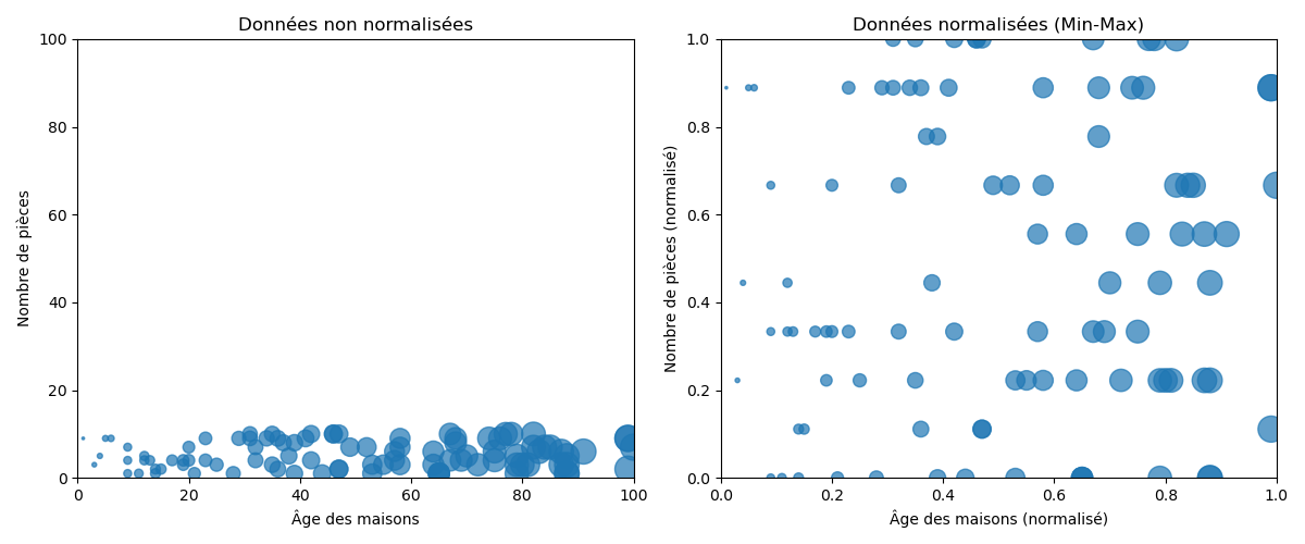
The process of normalization requires only the min and max, and the idea is to convert all values to a scale between 0 and 1 while preserving the distances between values.

$$X_{norm} = \frac{X - X_{min}}{X_{max} - X_{min}} \in [0, 1]$$

Normalization is recommended when the distribution of the data is unknown or when it is known that the distribution is not Gaussian ( bell-shaped ). It is preferred for algorithms that do not make assumptions about the data distribution, such as K-nearest neighbors or neural networks.

# Librairie Numpy
import numpy as np

def min_max_normalization(data):

 min_val = np.min(data)
 max_val = np.max(data)
 normalized_data = (data - min_val) / (max_val - min_val)
 return normalized_data

# Sickit-Learn Library
from sklearn.preprocessing import MinMaxScaler
import numpy as np

scaler = MinMaxScaler()
scaler.fit(data) # Calcul des Min & Max
normalized_data = scaler.transform(data)

normalized_data

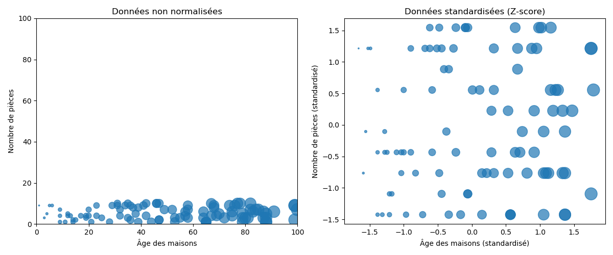
The process of standardization is more nuanced as it also aims to bring the mean to 0 and the standard deviation to 1.

$$Z = \frac{x_i - \bar{x}}{\sigma}$$

or:

$$Z = \frac{x_i - \bar{x}}{\sqrt{\frac{\sum_{i=1}^{n} (x_i - \bar{x})^2}{n}}}$$

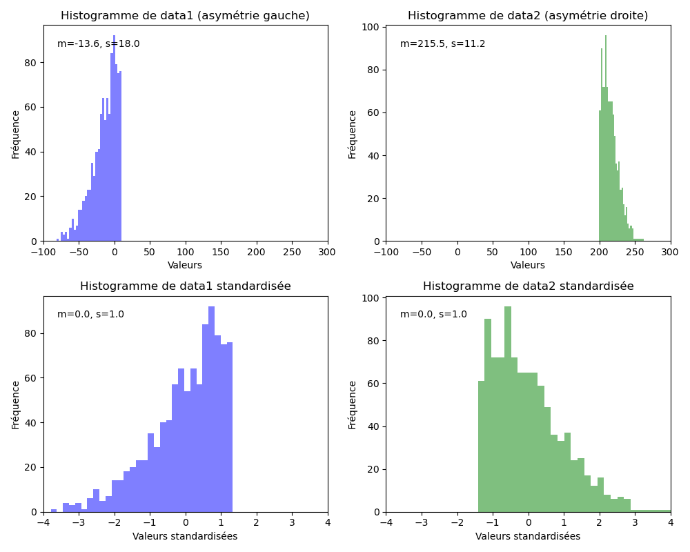
Standardization assumes that our data follows a Gaussian distribution ( bell curve ). While this does not have to be strictly true, the technique is more effective if it is.

The two distributions below are adjusted to a mean of 0 to align scales and avoid any bias.