Variable Selection

Variable selection involves choosing a subset of relevant variables from the full set of available variables in the data source. This step depends on :

• The objective of the data project ;
• Univariate statistical analysis of all variables ;
• The choice of the statistical technique to be applied and the variables required for creating the algorithm ;
• Specific statistical techniques ;
• The arbitrary choice of the data scientist ;
• ...

The Curse of Dimensionality

As data scientists, we must understand a crucial element regarding the expected qualities of a model, particularly its accuracy and calculation speed. These two elements will be strongly impacted by the choice of variables.

Most statistical techniques are executed by the CPU ( Central Processing Unit ) and use the computer’s RAM to store information. Some more resource-intensive techniques also use the GPU ( Graphics Processing Unit ), a graphics coprocessor that can lighten the CPU’s load. Some Python libraries are optimized for GPU usage. The idea behind variable selection is to pre-process the data to ensure efficiency.

Dimensionality corresponds to the number of columns x number of rows. It is important to understand that the more variables we use in an algorithm for applying a statistical technique, the more records are needed to ensure proper learning. Thus, dimensionality will be significant and, consequently, will impact computational performance.

Let’s take the following example - a chessboard - :

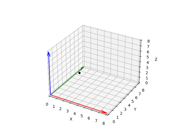
Imagine that the Y-axis is the ordinate ( numbers from $1$ to $8$ ) and the X-axis is the abscissa ( letters from a to h ). If we are limited by a chessboard to spread our data, we have the possibility of placing $64$ records. We are in two dimensions - we have selected two variables - $(x, y)$, and consequently, we have $64$ available squares. If we decide to add a third variable, the Z variable :

We increase the space from 64 squares to 512. However, it is important to understand that if we want to avoid underfitting, we need sufficient dispersion of records in this space. The rule is : the more variables we have, the more records we need.

But this must be carefully considered because :

• The more variables we include, the more complex the model will be, and the more records we will need to evaluate the relationships between variables.


• The higher the number of records, the more missing values will need to be addressed.


• The more variables there are, the higher the risk of having subsets of highly correlated variables. Including highly correlated variables can lead to issues of accuracy or reliability.

The goal is therefore to reduce the number of variables while ensuring that underfitting is avoided. Several options are available to the data scientist, such as (1) ignoring variables that are irrelevant to the objective ; (2) ignoring certain variables that are too highly correlated and whose simultaneous consideration would violate the hypothesis of non-collinearity ( linear independence ) of the explanatory variables ( predictors ) ; (3) using statistical techniques such as principal component analysis, forward selection / backward elimination - regression -, or applying a decision tree to identify the variables most correlated with the target variable.

Correlation

To understand correlation, it is important to recall the concept of variance and to define covariance. As we discussed in the univariate statistics section, variance is a measure of the dispersion of the values of a variable around its mean. It corresponds to the mean of the squared deviations from the mean and is always positive. It indicates whether a distribution is homogeneous or heterogeneous. In concrete terms, if variance is zero, it means that all the values of the records are equal to the mean - the distribution is perfectly homogeneous -. Variance is not interpretable on its own because it measures the squared deviation from the mean ( which is necessary to prevent positive and negative values from canceling each other out ), but the best indicator is, of course, the deviation from the mean, known as the standard deviation.

Variance is useful for comparing two variables together to characterize the simultaneous variations of two variables. This is referred to as covariance, which measures the strength of the relationship between two variables. In concrete terms, if two variables have significant covariance - for example, $70$ - this information highlights a linear relationship between the two variables. If we analyze the covariance between a predictor $x$ and the predicted variable $y$, we could then say that $x$ is a good predictor for $y$.

Formula for covariance: $s_{x,y} = \frac{\sum_{i=1}^{n} (x_i - \bar{x}) (y_i - \bar{y})}{n - 1}$

However, this is not entirely correct because covariance is not normalized and is therefore sensitive to units of measurement. It is important to consider the normalized form of covariance, known as correlation.

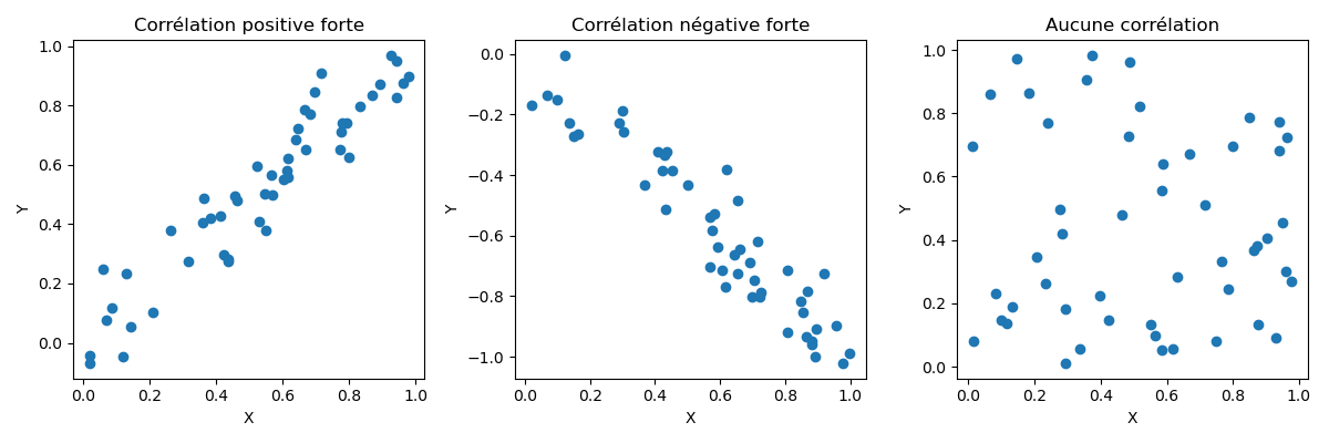
Correlation measures the strength and direction - whether positive or negative - between two variables. If one of the variables $x$ ( predictor ) has a high correlation with the target variable $y$, this indicates that this particular predictor strongly influences the target variable - it is therefore discriminant and very important for the model - and correlation also tells us whether this impact is positive or negative on the values of variable $y$.

Since correlation is normalized covariance, its value will always be between -1 ( perfect negative correlation ) and +1 ( perfect positive correlation ). A correlation of 1 means that an increase in variable A will have the same impact on variable B ( positive or negative ). Conversely, a correlation of 0 indicates the absence of a linear relationship between the two variables ( an increase in variable A has no impact on variable B ).

Formula for correlation : $r_{x,y} = \frac{\sum_{m=1}^{n} (x_{m} - \bar{x})(y_{m} - \bar{y})}{\sqrt{\sum_{m=1}^{n} (x_{m} - \bar{x})^2} \sqrt{\sum_{m=1}^{n} (y_{m} - \bar{y})^2}}$

We want to identify the variables $x$ most correlated with the target variable $y$. For example, the larger the area of a house, the higher the price ( strong influence as it is the most influential variable and positive direction as it increases the price ). Conversely, the higher the mileage of a car, the lower the price of the car. In this case, the variable « mileage » has a significant impact on the price ( strength ) and the direction is negative.

tip

To summarize : covariance is an extension of the concept of variance. Correlation is the normalized form of covariance. The more a variable $x$ is correlated ( positively or negatively ) with the variable $y$, the more important it is for our model as it is considered « discriminant ».

Collinearity

Collinearity is a situation where two variables are linearly associated ( highly correlated ) and are used as predictors of the target variable. This means that two variables $x ( x_1 and x_2 )$ are positively or negatively correlated and are used as predictors. This situation should be avoided because it makes it difficult to identify the independent effect of each $x$ variable on the predicted variable $y$.

For most techniques - except for neural networks - it is essential to avoid using correlated $x$ variables. Neural networks can handle this situation by adjusting weights, but decorrelating correlated variables still helps the algorithm converge to the optimal situation.

Multicollinearity

It is possible that two variables $x_1$ and $x_2$ are not correlated with each other, and individually, $x_1$ is not correlated with $x_3$, and $x_2$ is not correlated with $x_3$, but together, $x_1$ and $x_2$ are correlated with $x_3$. This is known as multicollinearity.

Techniques

As mentioned at the beginning of this chapter, our goal as data scientists is to optimize our models, making them as efficient as possible. Efficiency implies precision, speed, and robustness.

Feature Engineering

The first option for a data scientist is to apply feature engineering, which involves selecting and transforming the most relevant variables to optimize a model and achieve better performance. Feature engineering includes creating new variables based on existing ones, grouping variables into a new calculated variable, or transforming existing variables.

Let’s take the example of our real estate agency. The data available to predict house prices includes two variables : $x_8$ = lot width & $x_9$ = lot length. If we analyze $x_8$ and $x_9$ during the preparation stages, we should identify some positive correlation, and since these variables are used as predictors, we could say that we have a collinearity problem. In this example, one way to eliminate this collinearity is to create a new variable $x_10$ that would represent the lot area, with values corresponding to the multiplication of variables $x_8$ and $x_9$. $x_{10}$ would then be the final variable used as a predictor.

Applying Algorithms

There are specific algorithms that assist in variable selection. For example, forward & backward selection methods in regression techniques help identify the impact of adding and removing variables on the overall model evaluation.

The decision tree is a very useful statistical technique for helping select discriminant variables. Although it is also a supervised statistical technique - and therefore a predictive method - it can be used in the preparation algorithm of another prediction model. The decision tree technique prioritizes the separation of records by selecting, in the first node, the variable that best separates these records, i.e. the one that improves the purity score.

Principal Component Analysis ( PCA ) is a commonly applied unsupervised technique for selecting variables used as predictors that are correlated with each other. This technique redistributes the values of correlated variables into a new geometric space of smaller dimensions ( principal components ) by identifying the line that passes through most of the information between several variables, as well as subsequent perpendicular lines, allowing for the creation of uncorrelated principal components.