Principal Components

As we saw in the chapter on variable selection, the accuracy and calculation speed of a model are significantly impacted by the choice of variables used in a supervised or unsupervised model.

As a reminder, most statistical techniques are executed by the CPU ( Central Processing Unit ) and use the computer's memory ( RAM ) to store information. Some more resource-intensive techniques also rely on the GPU ( Graphic Processing Unit ), a graphics coprocessor that helps alleviate the CPU’s workload. The idea behind principal component analysis is to reduce data dimensionality to ensure a certain level of efficiency.

Dimensionality Recap

Dimensionality essentially refers to the number of columns multiplied by the number of rows. It is important to understand that the more variables we use in an algorithm for a statistical technique, the more records are needed to ensure learning. Higher dimensionality will affect computational performance and increase the risk of overfitting.

Variable selection/reduction is one way to reduce dimensionality. However, there are specific techniques for dimensionality reduction, among which principal component analysis is the most general, as it applies to both supervised and unsupervised algorithms.

Principal component analysis is therefore a dimensionality reduction method that reduces the number of variables studied ( fields / variables of a table ) while losing as little information as possible ( records ).

Linear Relationships

Principal component analysis can be applied in any case, but it is particularly effective when dealing with collinearity, i.e. correlation between predictors in a supervised technique.

Principal component analysis seeks to highlight strong linear relationships between variables, transforming them into new « decorrelated » variables that contain the majority of the information ( principal components ) and have a lower dimensional space ( variables and records ). This method is especially useful when the number of variables is large.

As a result, we obtain a limited number of variables corresponding to weighted linear combinations of the original variables, which retain most of the information from the original dataset.

Statistical & Geometric Transformation

This technique is both:

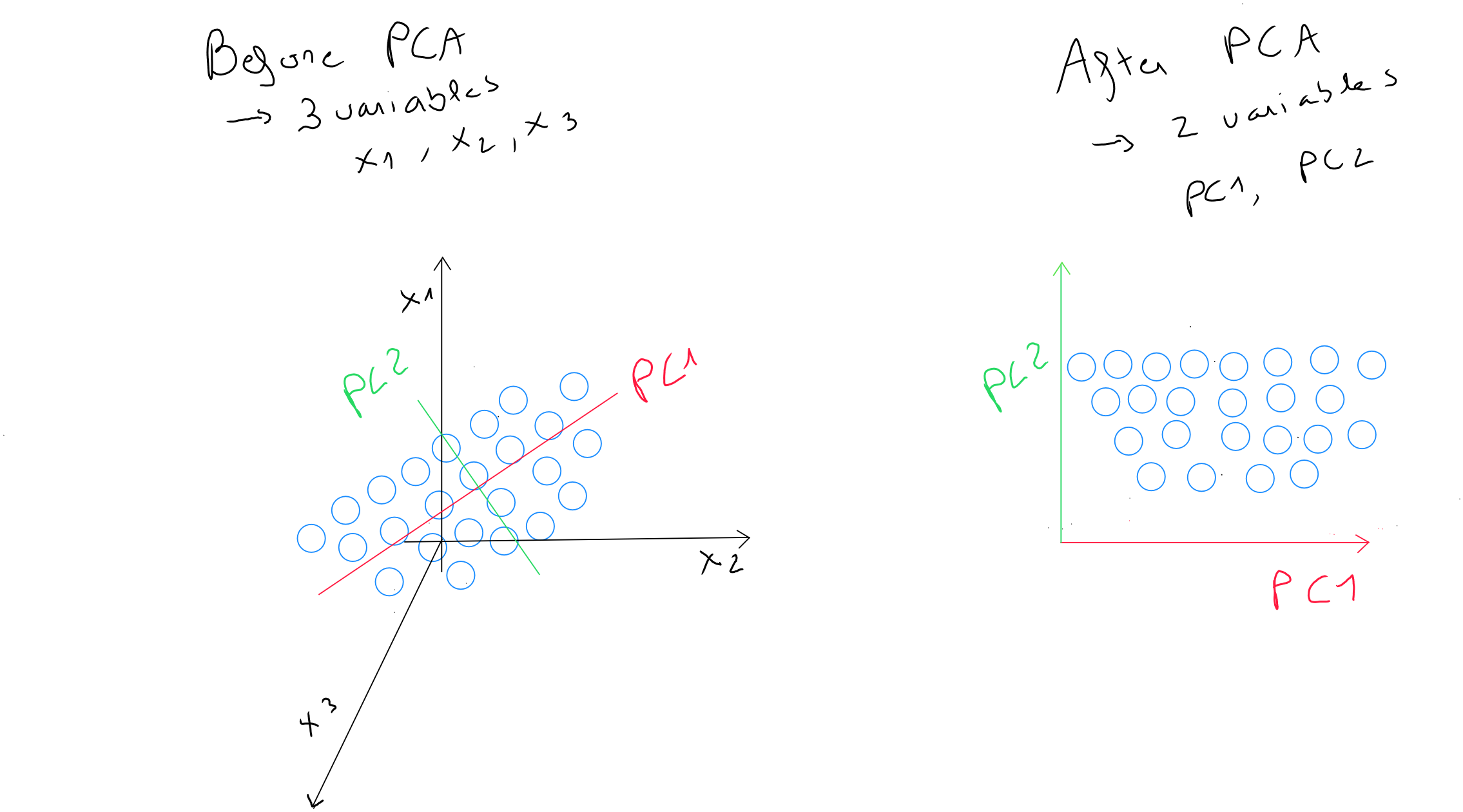
• Statistical : identifying the principal components, which are the directions that capture the majority of data variation ;
• Geometric : the space undergoes a rotation; points are projected into a new direction of lower dimensions while retaining the majority of the information from the original space ;

The statistical step involves identifying a linear combination of two variables that contains most - if not all - of the information. This linear combination is called $PC1$, the principal component, and replaces the two initial variables. The principal component represents the direction in which the variability of points is greatest. It is the line that captures the most variation in the data if we choose to reduce the dimensionality from $2$ to $1$. It is also the line that minimizes the sum of the perpendicular squared distances of the points to itself.

Next, we identify the line perpendicular to the first principal component that captures the second-largest variability among the points. By selecting the perpendicular to the first principal component $PC1$, we ensure that the second principal component $PC2$ is decorrelated.

The geometric step involves an orthogonal rotation of the axes to choose fewer components than the initial variables. The rotation only changes the coordinates of the points and allows the variability to be redistributed to capture as much information as possible.

For example, if our variables « weight », « height », and « age » contain the values $75$, $187$, and $35$, and they are redistributed into a new geometric space of two principal components PC1 and PC2, we may have two values of $148.5$ for PC1 and $-51.8$ for PC2. These two values differ from the three original values but still respect the same distance concept, and we have reduced our dimensionality by one axis.

Selecting Components and Variance

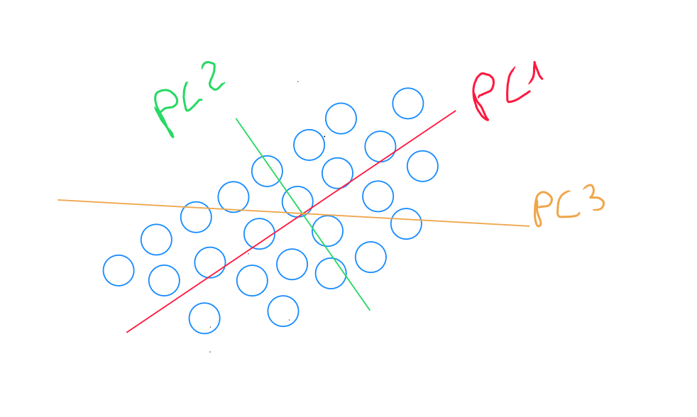
If we have many variables, identifying the third principal component explains the remaining variance in a dimension perpendicular to the first two principal components. Consequently, the variance captured by PC3 is smaller than that captured by PC1 and PC2, but it is still present. PC3 captures the variations not aligned with the directions of PC1 and PC2. Identifying additional components follows a similar process as before.

The amount of variance explained by each principal component allows us to determine the optimal number of components, representing the cumulative proportion of data variance after adding each principal component.

For example, in a model with 20 variables, it may be that by the second principal component, $99$ of the data's variance is captured, reducing the dimensional space from $20$ variables to $2$ components.

Python Code

In preprocessing, all data must be digitized, either through one-hot encoding or by using the discretization of discrete variables process.

data = pd.read_csv('data.csv')

pcs = PCA()
pcs.fit(data.dropna(axis=0))
pcsSummary= pd.DataFrame({'Standard deviation': np.sqrt(pcs.explained_variance_),
                         'proportion of variance': pcs.explained_variance_ratio_,
                         'cumulative proportion': np.cumsum(pcs.explained_variance_ratio_)})
pcsSummary = pcsSummary.transpose()
pcsSummary.columns= ['PC{}'.format(i) for i in range(1,len(pcsSummary.columns)+1)]
pcsSummary.round(4)

pcsComponents_df = pd.DataFrame(pcs.components_.transpose(),columns=pcsSummary.columns,index=data.columns)
pcsComponents_df