Neural Networks

The idea behind a computer neural network is to take inspiration from the functioning of the human brain. It is a statistical technique conceptualized in the late 1950s within the framework of a supervised binary classification learning algorithm, which has seen various evolutions in subsequent years ( e.g. recurrent neural network models, multilayer perceptron, etc. ).

Neural networks were heavily used in the late $80$s and early $90$s due to their ability to process unstructured data, particularly handwritten recognition. At that time, its usefulness was demonstrated in sorting mail for postal services and identifying monetary symbols on checks.

Despite its achievements, it was only from the 2000s to 2010 that this technique - rebranded Deep learning - re-emerged and showed high capabilities in revolutionary concepts such as image recognition or voice recognition. This resurgence is mainly attributed to two factors : on the one hand, the hardware evolution, particularly the use of GPUs ( Graphic Processing Units ) - which are particularly powerful for vector computations ; and on the other hand, the increasing availability of large datasets. Researchers realized that the more data they fed a model, combined with a large architecture enabled by computational capacity, the more remarkable the performance became.

The term Deep learning ( deep learning ) - which appeared around 2005 - is primarily related to the architecture's characteristic of neural networks ; The « black box of hidden layers ».

To understand a computer neural network, it is important to grasp the fundamentals of a biological neural network.

note

Some of the diagrams and concepts presented here are inspired by the Machine Learning course by Andrew Ng, a program created in collaboration between Stanford University Online Education and DeepLearning.AI, available on Coursera. Find the original course here: Machine Learning by Andrew Ng.

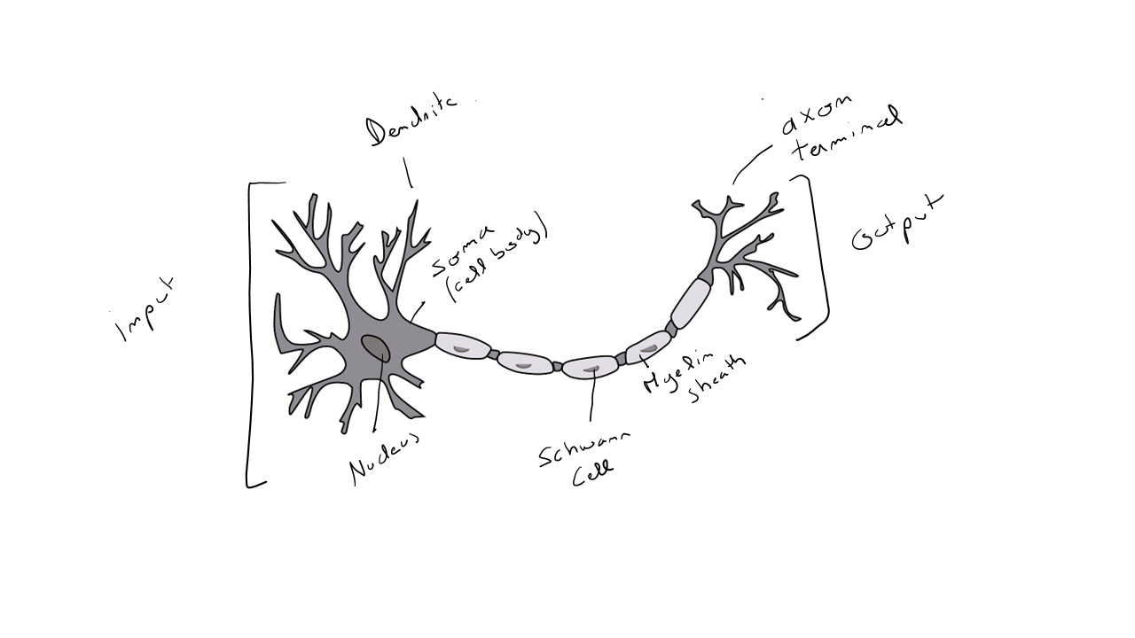
Representation of a neuron :

Representation of a computer neuron :

A human has about $86$ to $100$ billion neurons in the brain. The role of a neuron - a brain cell - is to transmit information and enable motor and cognitive activities. Specifically, if you turn a corner and face a lion that has escaped from a zoo, your neurons will activate : identifying and understanding the danger, associating the situation with many pieces of information and possible reactions, accelerating the heart rate to increase blood flow to your limbs and prepare for a potential motor escape ( although it is recommended not to move ! ), etc.

Neurons communicate with each other through electrical signals ( nerve impulses ) and are connected via dendrites and axons. A neuron receives information from another neuron through an incoming electrical signal via dendrites. The signal propagates along the neuron's axon and is then sent to another neuron, which activates in turn. Axons are surrounded by a myelin sheath that accelerates nerve impulse conduction. The higher the frequency of the electrical signal, the more neurotransmitters are produced by the neuron, which enables communication with other neurons through synapses. The neural environment, within the nervous system, consists of glial cells ( 50 % of brain volume ) that provide nutrients and oxygen while also eliminating dead cells.

Humankind has always drawn inspiration from nature for many advances. While we will explore the power of this statistical technique, it is crucial to emphasize an important point : if we want to create artificial intelligences as strong as humans - ( and note that intelligence takes various forms such as logic, self-awareness, learning, creativity, emotion, etc. ) - we would need to fully understand how the human brain works, which is not yet entirely the case. For example, recent research increasingly highlights the essential, non-reproducible roles of glial cells and myelin from an IT perspective.

However, if we refer to the basic functioning of a neuron, it could be summarized as follows : an input layer receives one or more pieces of information via dendrites in the form of electrical flow ; the electrical flows are activated at a certain density through the axon to produce an output ( electrical flow ), which will serve as input information for another neuron.

It is interesting to draw a parallel with how a computer operates, which is essentially made up of numerous transistors orchestrated by the Central Processing Unit ( CPU ), controlling the intensity of an electrical signal using three operators : AND, OR, and NOT. These conditions are represented by the presence ( 5 volts ) or absence of an electrical current, ultimately expressed as either 1 or 0.

Neural Networks & Linear/Logistic Regression

The process of a computer neural network is also relatively simple : we have one or more input data, this data is processed in a layer based on activation functions, and we obtain an output value.

Zooming in on a computer neuron, we discover that a logistic regression or a linear regression ( depending on the activation function ) is actually a simplified model of a neuron :

$x$ = values of the explanatory variable (predictor)

$a$ = activation function ( output value elevation measure ) $= f(z) =  \frac{1}{1 + e^{(-(w *x + b))}}$ = probability or $\hat{Y} = b + w * x$ estimation

tip

A computer neural network could be considered a network of a set of linear and / or logistic regressions ; the techniques are defined based on an activation function per layer ( Linear, Logistic, ReLu, Softmax ).

To illustrate how a neural network works, consider the following prediction case : a shoe seller asks for our help to predict if a new sneaker model will be a top seller or not to ensure optimal stock management and decide if the sneakers should be included in their upcoming month's promotional flyer.

$\hat{y}$ corresponds to Top Seller $(1)$ or not Top Seller $(0)$. It is therefore a supervised classification technique. If we have only one predictor $x =$ price ; we might define that the best model to use is simple logistic regression, and we could make the following association between a neuron ( a unit of a neural network ) and our logistic regression :

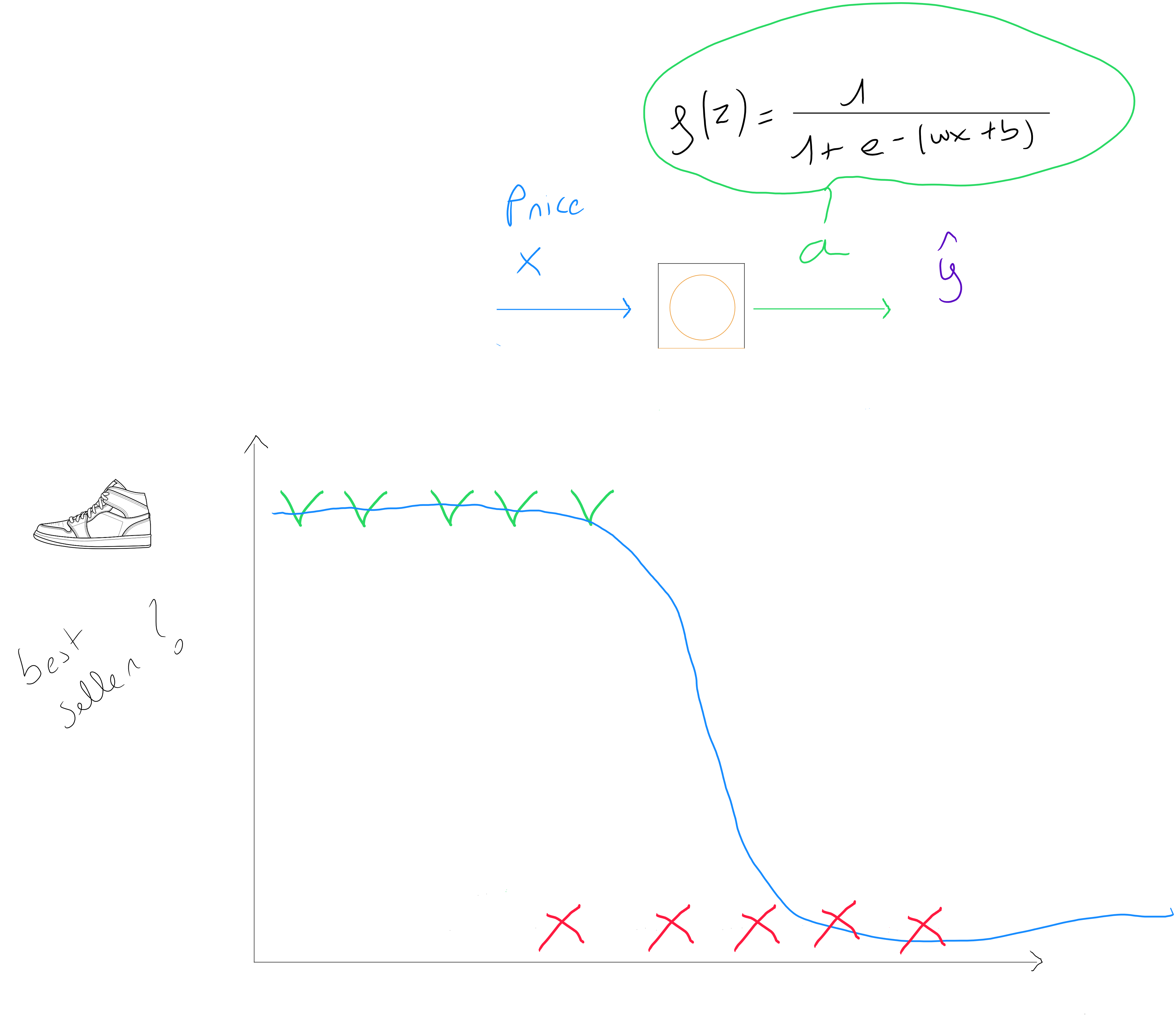
If we had several predictors, we would apply the following logistic regression function for multiple predictors : $f(z) = \frac{1}{1 + e^{(-(\vec{w} \cdot \vec{x} + b))}}$. In practice, this means that a neural network will estimate parameter values for $w$ and $b$ for each neuron in each layer of the network.

If we decide to use a neural network with several predictors :

Price	Delivery Cost	Marketing Fees	Material (Quality)	Top Seller
80 €	5 €	10 €	9	1
50 €	2 €	8 €	6	0
120 €	8 €	15 €	9	1
65 €	3 €	6 €	4	0
...	...	...	...	...
95 €	7 €	12 €	3	1

Neural Network Architecture

The key feature of a neural network - its architecture - is that it consists of what is called an input layer, one or more hidden layers, and an output layer. The input and output layers are visible, as they respectively represent the predictor values $\vec{x}$ and the predicted variable $\hat{y}$.

However, as data scientists, we cannot see what happens inside a hidden layer. This is known as the « black box ». It is by no means a form of machine intelligence - as we will discuss later - but rather, hidden layers function through error gradient backpropagation.

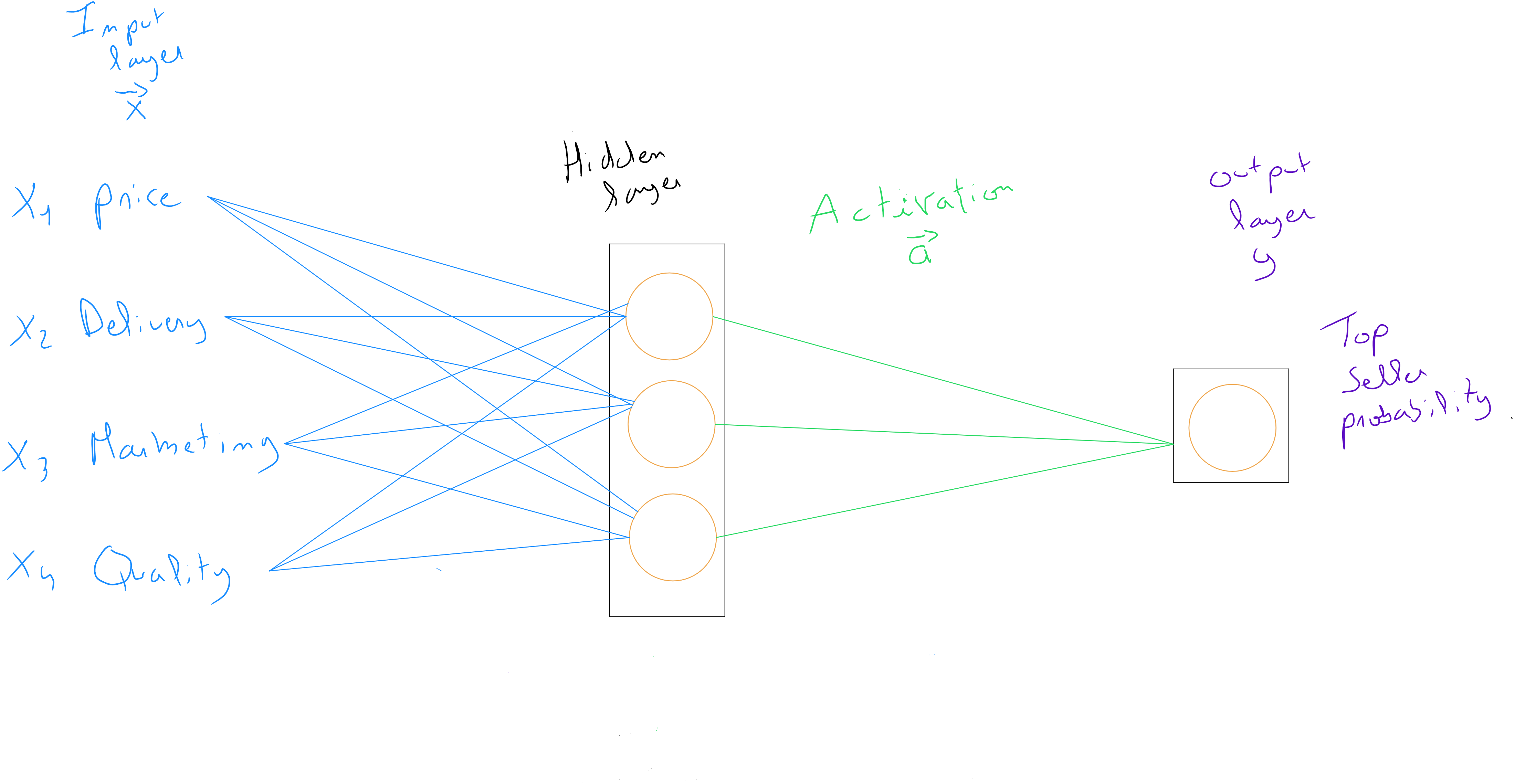
Even though all $x$ values are used as input values in each hidden layer neuron in the above example, it’s essential to understand that during its learning process, the model can potentially deactivate variables or reduce the impact of some variables based on the weight definitions $w$.

If we had access to how the model operates in the hidden layer in our example, we might discover that it groups the input variables into three criteria ( represented by $3$ neurons ), such as affordable price, brand reputation, and perceived quality. For the reputation factor, while the neuron receives information about delivery costs, these might have little impact on reputation and may be almost nullified by the weight ; whereas price and marketing efforts have a significant influence. Finally, the values of these three neurons are reused as inputs for the last neuron, which, based on this information, defines the probability of being a top seller.

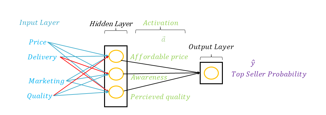
A neural network can have many hidden layers, in which case we refer to it as an MLP, or Multi-Layer Perceptron. As data scientists, we must make an important decision : to initiate different neural network architectures, which will be evaluated to identify the most efficient one.

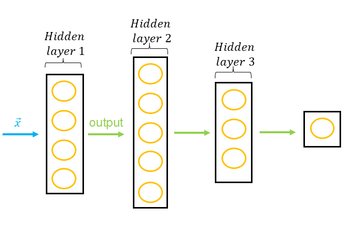
A neural network can be used for classification or estimation, and it requires quantitative or qualitative predictors that have been transformed through one-hot encoding or digitizing discrete variables. To ensure efficiency, the data must be normalized before being split into a training set and a validation set.

As data scientists, we must define the architecture of our neural network, meaning the number of hidden layers and the number of neurons per layer. In practice, multiple architectures are evaluated. For instance, if we have $8$ predictor variables $x$, we might define three architectures as follows :

• Input layer = 8; Layer_1 = 16; Layer_2 = 32; Layer_3 = 16; output layer = 1
• Input layer = 8; Layer_1 = 32; Layer_2 = 16; output layer = 1
• Input layer = 8; Layer_1 = 64; Layer_2 = 32; Layer_3 = 16; Layer_4 = 4; output layer = 1

We could also test different activation functions between layers for these three architectures ( sigmoid, linear, ReLU, softmax - see the activation functions section - ) as well as various learning rates and batch sizes ( splitting data into smaller subsets for parameter updates ).

Each configuration will be trained, and the final model with the best efficiency will be selected.

Building a Layer

As we discussed earlier, a layer groups a set of neurons, and each neuron can be considered as a linear and / or logistic regression depending on the activation function. As data scientists, we need to identify the most efficient architecture, which means determining the number of layers and neurons per layer.

The difference between a logistic / linear regression and a neuron is that the final output value obtained by a neuron is considered as the result of the activation function ( which equals the logistic or linear function ( sigmoid, Linear, ReLU, or Softmax derivatives) ).

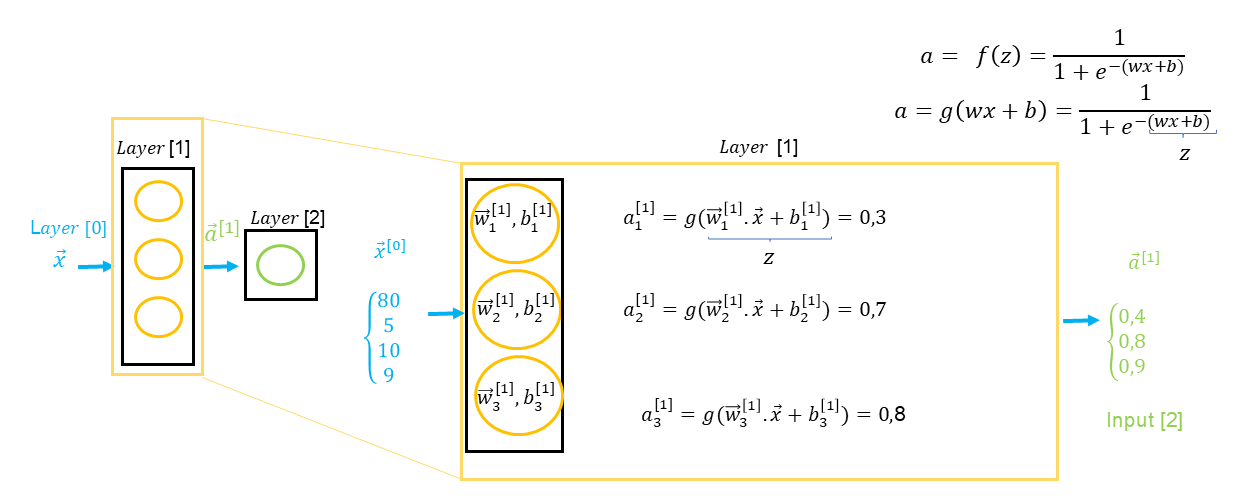
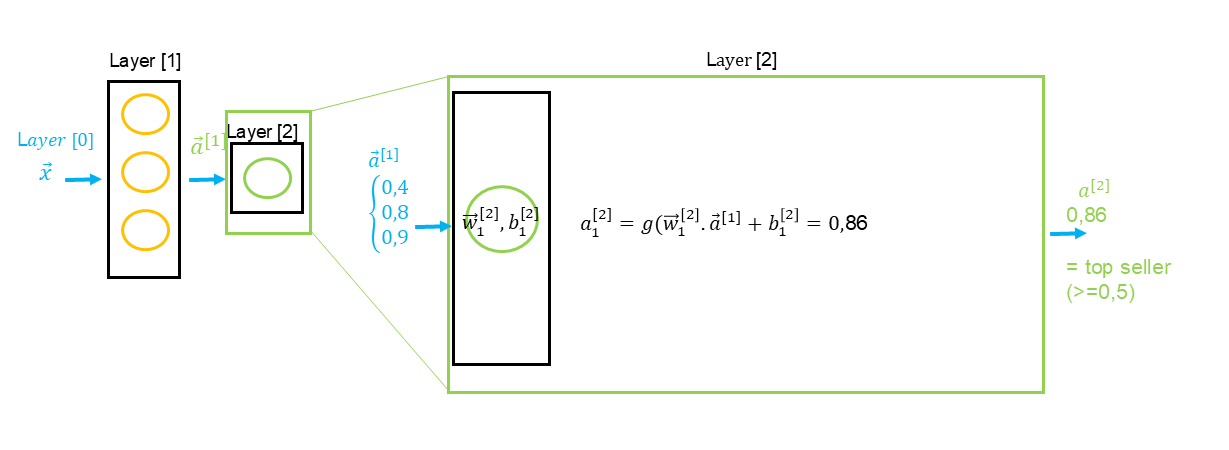
The result of layer $2$ is a vector $a$ containing each neuron’s output values. In the example above, we see that the input layer corresponds to a vector $x$ ($\vec{x}$), meaning values for each predictor ( price $X_1$, delivery cost $X_2$, marketing costs $X_3$, and quality $X_4$ ). The result is a vector $a$ ($\vec{a}$) representing the output values of each neuron, such as $a_1^{[1]},a_2^{[1]},a_3^{[1]}$, which will then become input values for the next layer, and so on until the final layer.

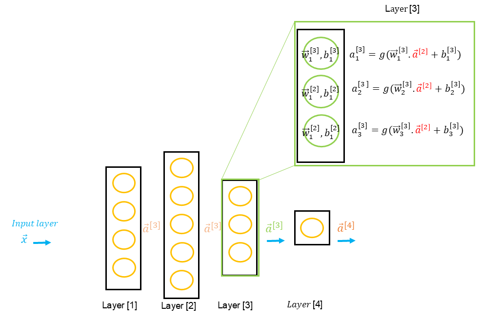
If we have a second hidden layer, it’s important to note the particularities of the formula annotations regarding input data from the previous layer : g(z) = g(\vec{w} \cdot \textcolor{red}{\vec{a^{[Layer -1]}}} + \)b

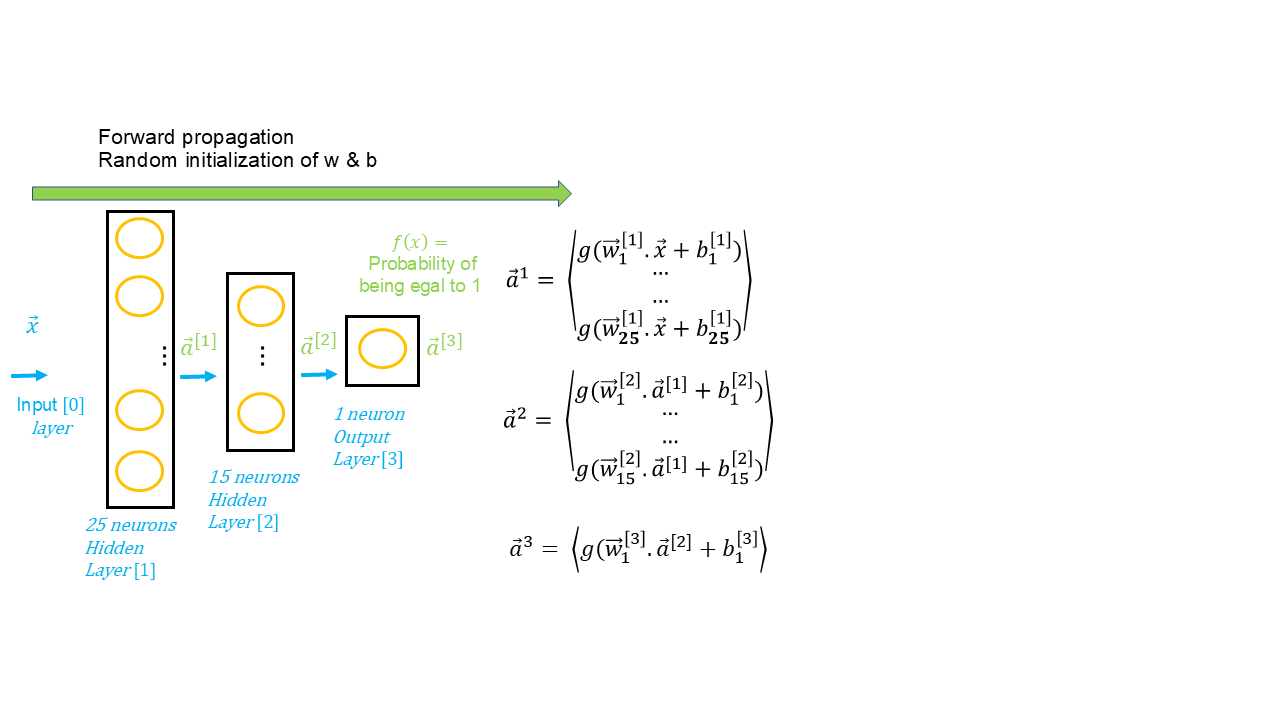
Forward Propagation

Forward propagation is the initial step in building a neural network model. Let’s recall that all the data preparation steps and defining the neural network architecture concern the algorithm. Once these steps are ready, it’s time to launch the model. The model refers to applying the algorithm to data and evaluating the entire process.

We refer to it as forward propagation because the data is propagated forward from the input layer, through the hidden layers, and finally to the output layer, the final result. Each layer includes a set of neurons ( each unit being a sort of linear or logistic regression ), and activation functions are defined for each layer. Generally, the same activation function is used for hidden layers, and either the same or a different function is used for the output layer.

Therefore, forward propagation involves passing the data through various layers, assigning an output value at each step based on an activation function, until reaching the final prediction.

Of course, we saw in the context of linear and logistic regression that the objective of a supervised algorithm is to predict values based on a cost function and apply an optimization algorithm to minimize this cost by identifying the values of $w$ and $b$. Neural networks work the same way because they are parametric techniques. As in the initialization of linear or logistic regression, random values are set for $w$ and $b$ during the first iteration ; in this case, during forward propagation.

Backward Propagation

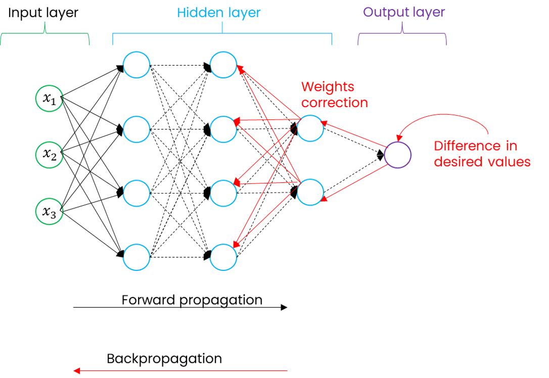
Once predictions are made through forward propagation and random initialization of $w$ and $b$ parameters, the neural network algorithm also includes the concept of a cost function. It will use an algorithm to minimize the cost function by finding the local optimum, meaning identifying the values of $w$ and $b$ that minimize the differences between the predicted and actual values.

Backward propagation consists of retracing through the network’s layers, but this time in reverse, to adjust the values of $w$ and $b$ for each neuron in each layer. In the diagram below, forward propagation is represented in blue and backpropagation in red.

Cost Function

We have seen that a neural network is similar - for each neuron as a unit - to a linear and / or logistic regression. In the first step, we apply forward propagation, meaning the application of the algorithm to our data based on randomly initialized parameters.

As a result, we will observe fundamental differences between the actual known values of the training set and the predicted values from our first iteration ( epoch ). To identify these errors, a neural network uses a cost function for each neuron ( each neuron having an associated $b$ and $w$ parameter ). This cost function is identical to linear regression for an estimation neural network and to logistic regression for a classification neural network, as follows :

For linear regression

$$J(w, b) = \frac{1}{2m} \sum_{i=1}^n ((w \cdot x^{(i)} + b) - y^{(i)})^2$$

For logistic regression

$$J(\vec{w}, b) = -\frac{1}{m} \sum_{i=1}^n y^{(i)}log(f(\vec{w},b)\vec{x}^{(i)}) + (1-y^{(i)})log(1-f(\vec{w},b)\vec{x}^{(i)})$$

Gradient Descent & Adam

Of course, the cost function allows us to identify the differences between actual and predicted values, but just like in linear and logistic regression, we need an algorithm to find the local optimum, which means minimizing the cost function by identifying the values of $w$ and $b$ that will yield the best predictions.

Previously, we discussed the steps of the gradient descent algorithm, which involve applying the cost function, calculating the derivatives of $w$ and $b$ to determine how to update the parameters at each iteration of the algorithm ( whether to increase or decrease their values ).

We also noted that during the application of these derivatives, we must, as data scientists, provide a fixed alpha value $α$, which, when combined with the derivatives, defines the « step size » for moving toward the local optimum. This step size will decrease as we approach the optimum. The problem with this alpha value $α$ is that we do not know in advance the best value for our model, so we often test several options: $(0.1; 0.03; 0.01; 0.003; 0.001; etc. )$. If alpha takes steps that are too large, it risks missing the local optimum, and in this case, we see the $w$ and $b$ values adjust in the opposite direction.

tip

Gradient Descent

$J(w, b) = \frac{1}{2m} \sum_{i=1}^n ((w \cdot x^{(i)} + b) - y^{(i)})^2$

1. $temp_w = w - \alpha \frac{d}{dw} J(w, b) = w - \alpha \frac{1}{m} \sum_{i=1}^{m} [f_{w,b}(x^{(i)}) - y^{(i)}] x^{(i)}$ ;
2. $temp_b = b - \alpha \frac{d}{db} J(w, b) = b - \alpha \frac{1}{m} \sum_{i=1}^{m} [f_{w,b}(x^{(i)}) - y^{(i)}]$ ;
3. $w = temp_w$ ;
4. $b = temp_b$ ;

Adam - Adaptive Moment Estimation - is an algorithm that functions similarly to gradient descent, except it doesn’t use a single alpha value $a$. Instead, it uses different values for each parameter in our model, meaning different values for each neuron. It is therefore considered an adaptive optimizer of gradient descent that adjusts the learning rate for each parameter, providing faster and more stable convergence.

For example, if our model has 15 $w$ values :

$$temp_{w1} = w_1 - \alpha_1 \frac{d}{dw_1} J(w, b)$$$$...$$$$temp_{w15} = w_{15} - \alpha_{15} \frac{d}{dw_{15}} J(w, b)$$$$temp_b = b - \alpha_{16} \frac{d}{db} J(w, b)$$

In this case, each alpha will be different, and Adam will adjust them as the training progresses, considering that if smaller alpha values help early parameters move in a certain direction, those alpha values may continue to increase more significantly for the later parameters, leading to faster local optimum convergence. Conversely, Adam may also begin to reduce step sizes significantly.

Epochs

An epoch represents one complete cycle through the training data for a neural network.

An epoch consists of three phases :

• Phase 1: Forward propagation
• Phase 2: Application of the cost function and error calculation
• Phase 3: Backpropagation to adjust the weights based on the error gradient

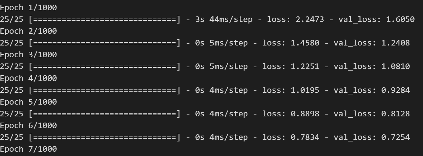
As data scientists, we must arbitrarily define the number of epochs. This is what is known as a hyperparameter. It determines how many times the entire training dataset will be presented to the network for learning.

Typically, we set a large number of epochs, and we include what is called an « early stop » in the algorithm, meaning an early stop based on the reduction in cost calculated at each iteration. For example, we specify that if the cost does not decrease by a certain value ( e.g., < 0.000001 ), then the model is sufficiently trained.

Batch Size

The batch size is also a hyperparameter that we must specify during the training of a neural network model. This is a particular feature of neural networks, which are often used when the training data is large. Therefore, most code editors and libraries associated with neural networks are designed to take full advantage of GPU ( Graphic Processing Unit ) computing.

In practice, applying a batch size consists of subdividing the training data into smaller learning samples, which are processed in one iteration of gradient descent ( or Adam ). Using a batch size on large datasets improves computational efficiency and allows faster convergence while also preventing overfitting.

The recommended values are usually powers of 2: 32, 64, 128, 256, 512, 1024, 2048, because GPUs are optimized for powers of $2$. Generally, smaller values ( 32 or 64 ) are chosen to improve generalization, but it's important to note that a larger batch size - which requires more GPU memory - allows for faster training.

Activation Functions

In a neural network, we have seen that each neuron has its own $w$ and $b$ parameters. We will see in the following section that when building a neural network in Python, we define an activation function for each layer. An activation function is somewhat like determining for each neuron layer whether the network should apply logistic or linear regression. Of course, it's a bit more complex than that since there are other functions - more evolved - that allow faster computations, thus making the neural network more efficient.

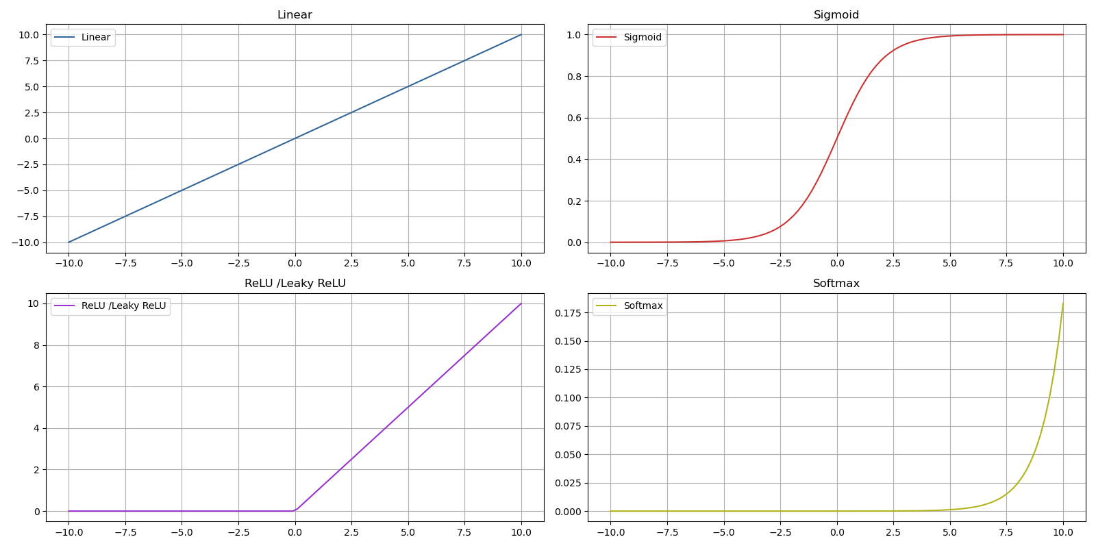
The most common activation functions today are :

• ReLU - Rectified Linear Unit - : this function is the most used for hidden layers in a neural network because its computation is simple and therefore fast ( faster convergence compared to other functions ), and it especially avoids gradient saturation for positive values ;
• Leaky ReLU : a variant of ReLU that avoids neurons being deactivated by the ReLU function by ensuring that even if a neuron receives a negative input, it can still output a very small but non-zero value ;
• Sigmoid : this function is more commonly used in output layers or for all layers in a binary classification problem, as in other cases its convergence is slower than ReLU ;
• SoftMax : a function used in the output layer for multiclass classification and allows interpretation of multiple classes based on probabilities ;
• Linear : this function is mainly used in the output layer for an estimation problem ;

The activation functions Tanh, SoftmaxPlus, and Elu are less commonly used nowadays and are therefore not included in this document.

Complete Python Code

The following code is used for estimation.

For classification, the following principles must be changed :

• Output layer activation function ( sigmoid for binary classification, softmax for multiclass classification ) ;
• The cost function in model.compile ( 'binary_crossentropy' for binary classification and 'categorical_crossentropy' for multiclass classification ) ;
• The evaluation metric in model.compile : metrics=['accuracy'] ;

Finally, in the case of multiclass classification, $y$ must be represented in one-hot encoding to obtain as many $y$ as there are classes. The prediction will then define a probability for each $y$ ;

import pandas as pd
import tensorflow as tf
from tensorflow.keras.models import Sequential
from tensorflow.keras.layers import Dense
import numpy as np
from sklearn.preprocessing import StandardScaler
from sklearn.model_selection import train_test_split
from sklearn.metrics import mean_squared_error


data = pd.read_csv('data.csv')
x = data[['x_1', 'x_2', 'x_3', 'x_4', 'x_n']].values  
y = data['y'].values  

scaler_x = StandardScaler()
scaler_y = StandardScaler()

x = scaler_x.fit_transform(x)
y = scaler_y.fit_transform(y.reshape(-1, 1))

x_train, x_test, y_train, y_test = train_test_split(x, y, test_size=0.4, random_state=42)

def build_models():
    tf.random.set_seed(20)
    
    model_1 = Sequential([
        Dense(8, activation='relu', input_shape=(x_train.shape[1],)),
        Dense(4, activation='relu'),
        Dense(1, activation='linear')
    ], name='model_1')

    model_2 = Sequential([
        Dense(16, activation='relu', input_shape=(x_train.shape[1],), kernel_regularizer=tf.keras.regularizers.l2(0.01)),
        Dense(8, activation='relu', kernel_regularizer=tf.keras.regularizers.l2(0.01)),
        Dense(1, activation='linear')
    ], name='model_2')

    model_3 = Sequential([
        Dense(32, activation='relu', input_shape=(x_train.shape[1],), kernel_regularizer=tf.keras.regularizers.l2(0.01)),
        Dense(16, activation='relu', kernel_regularizer=tf.keras.regularizers.l2(0.01)),
        Dense(1, activation='linear')
    ], name='model_3')

    model_4 = Sequential([
        Dense(64, activation='relu', input_shape=(x_train.shape[1],), kernel_regularizer=tf.keras.regularizers.l2(0.01)),
        Dense(32, activation='relu', kernel_regularizer=tf.keras.regularizers.l2(0.01)),
        Dense(16, activation='relu', kernel_regularizer=tf.keras.regularizers.l2(0.01)),
        Dense(1, activation='linear')
    ], name='model_4')
    
    model_list = [model_1, model_2, model_3, model_4]
    
    return model_list


nn_models = build_models()


for model in nn_models:
    model.compile(
        loss='mse',
        optimizer=tf.keras.optimizers.Adam(learning_rate=0.01)
    )
    
    print(f"Training {model.name}...")
    
    model.fit(
        x_train, y_train,
        epochs=1000,
        batch_size=32,
        validation_split=0.1,
        verbose=0
    )
    
    print("Done!\n")


    yhat_train = model.predict(x_train)
    yhat_test = model.predict(x_test)
    
    rmse_train = mean_squared_error(y_train, yhat_train, squared=False)
    rmse_test = mean_squared_error(y_test, yhat_test, squared=False)
    
    print(f"Model {model.name} - RMSE on Training Set: {rmse_train:.4f}")
    print(f"Model {model.name} - RMSE on Test Set: {rmse_test:.4f}\n")

Prediction for a New Record :

X_new = [[0, 0, 0, 0, 0]]  

X_new_scaled = scaler_x.transform(X_new)

y_new_scaled = model.predict(X_new_scaled)

y_new = scaler_y.inverse_transform(y_new_scaled)
print(y_new)