KNN Nearest Neighbors

The k-nearest neighbors ( K-NN ) technique is a highly automated, non-parametric supervised learning method that can be used for :

• Classification : a categorical variable assigned to the new record based on the vote of the most frequent values among the nearest neighbors ;
• Prediction : a continuous variable defined based on the ( weighted ) average of the values of the nearest neighbors ;

This technique is based on the concept of similarity, identifying similar records in the dataset to assign a missing value to a record based on the values of its nearest neighbors.

Basic Principles

« If it looks like a duck, swims like a duck, and quacks like a duck, then it probably is a duck ! »

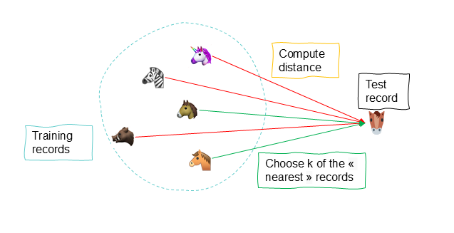
We identify the $k$ most similar records ( nearest neighbors ) based on common predictors and a distance calculation of the values, allowing us to assign the target variable $( y_i )$ to the new record based on the existing values $( y_n )$ of the nearest neighbors.

Unlike linear regression, the K-NN algorithm is a method that does not consider potential relationships between the target variable $( 𝑦 )$ and the predictors $x_[𝑖1],x_[𝑖2],.. x_[ip]$. It is a non-parametric method because it does not involve estimating parameters to define an assumed function form, as is the case for the linear form of linear regression. Instead, this method draws information from similarities between the predictor values of records in the dataset.

Let’s take the following example of car data :

Price	Age	Power	Weight	Km	Tax €	Diesel	Gasoline
13,500	23	90	1165	46,986	210	1	0
14,950	26	90	1170	48,000	224	1	0
22,950	30	150	1220	34,000	150	0	1
12,950	32	80	1050	?	215	1	0

The data lacks a value for mileage for the fourth record. The K-Nearest Neighbors ( K-NN ) method will search, based on the predictors ( other common variables ) and a distance calculation, for the $k$ similar records ( neighbors ) with known values for the target variable ( KM ). Based on this information, and by applying a weighted average, we can predict the mileage for this vehicle.

When we talk about similarity in data, it always refers to proximity, meaning the calculation of the distance between one record and another. Specifically, the algorithm will calculate the proximity order of the existing records with known KM values and the record for which we want to identify the value.

For the record for which we are looking for the KM value, the price is $12,950$. The algorithm will calculate the distances as follows : distance1 = $\sqrt{(12,950 - 13,500)^²}$ ; distance2 = $\sqrt{(12,950 - 14,950)^²}$ ; and so on.

For classification, the method is similar. We also identify the dominant class value among the $k$ nearest records, which is then assigned to the record with the missing information.

Price	Age	Power	Weight	Km	Tax €	Fuel Type
13,500	23	90	1165	46,986	210	Diesel
14,950	26	90	1170	48,000	224	?
22,950	30	150	1220	34,000	150	Gasoline
12,950	32	80	1050	47,500	215	Diesel

Distance Concepts

To identify the nearest neighbors, this method draws information from similarities between the predictive values of records in the dataset, considering the notion of distance. The central question is how to measure the distances between records based on predictive values. What makes these properties useful is the fact that a well-defined distance implies that every record has a neighbor among the other data.

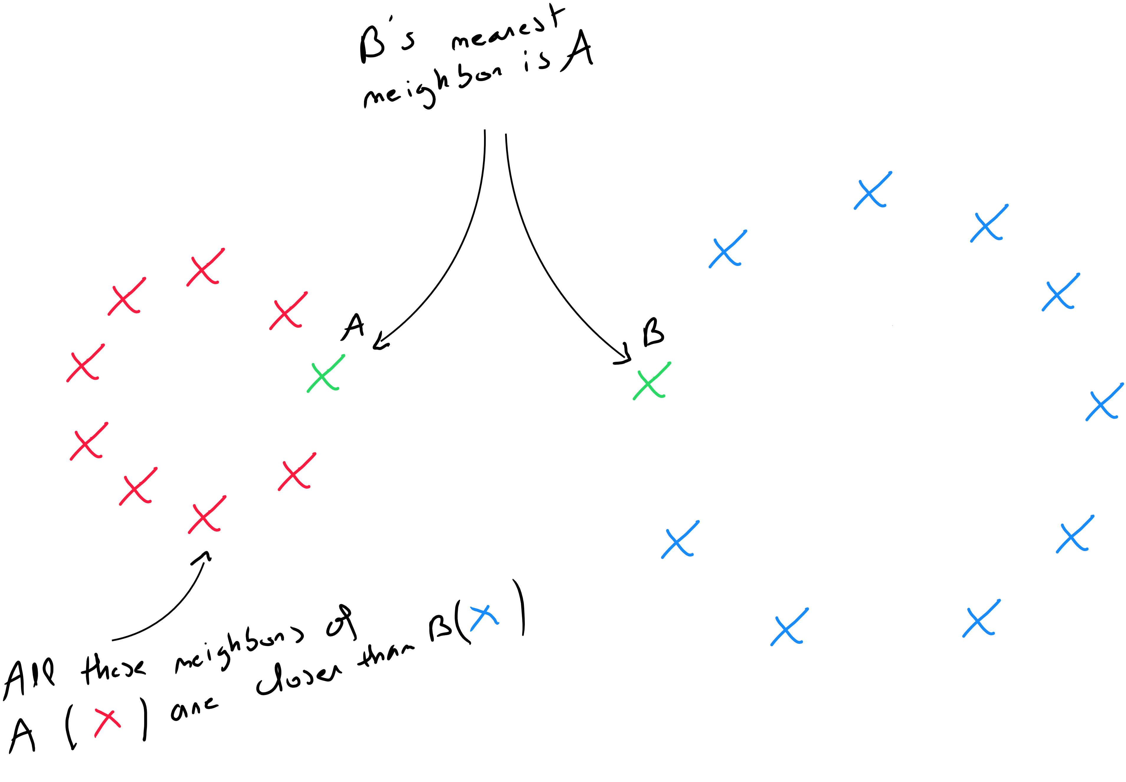
The distance of a record from another must be calculated based on all the different types of predictors. However, one of the fundamental concepts is to transform the data to apply distance calculations. If the variables are ordinal qualitative, they must be digitised. If the variables are nominal qualitative, we must apply one-hot encoding.

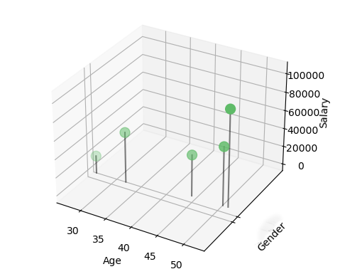
In this case, the distance will be calculated for each field. Let’s take the example of the following dataset, which contains two quantitative variables and one qualitative variable :

ID	Gender	Age	Salary
1	Female	27	19,000
2	Male	51	64,000
3	Male	52	105,000
4	Female	33	55,000
5	Male	45	45,000

A three-dimensional scatter plot helps us better identify the distances between records. The idea is to calculate the distance between all the values of one record and the values of the other records, then determine, based on a threshold, the $k$ nearest neighbors.

Euclidean Distance

Euclidean distance is the most commonly used to calculate the distance between two records, as it is considered the most efficient. It is simply the most direct distance between point A and point B.

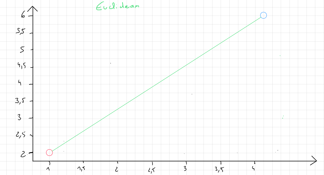
The formula for Euclidean distance is written as follows :

$$d(p, q) = \sqrt{\sum_{i=1}^{n} (p_i - q_i)^2}$$

or

$$d(p, q) = \sqrt{(p_{i1} - q_{i1})^2 + (p_{i2} - q_{i2})^2 + \dots + (p_{in} - q_{in})^2}$$

For the following example :

ID	$x_1$	$x_2$	$x_3$	$x_4$	$x_5$	$x_6$	$x_7$	$x_8$
01	1.06	9.2	151	54.4	1.6	9.077	0	0.628
02	0.89	10.3	202	57.9	2.2	5.088	25.3	1.555

The distance is calculated as follows :

$$d_{1,2} = \sqrt{(1.06 - 0.89)^2 + (9.2 - 10.3)^2 + (151 - 202)^2 + (54.4 - 57.9)^2 + (1.6 - 2.2)^2 + (9.077 - 5.088)^2 +(0.628 - 1.555)^2 } = 3989.408$$

The distance is calculated for all records $d_{1,3},d_{1,4},d_{1,...},d_{1,n}$.

Euclidean distance is strongly influenced by the scale of each variable, so it is customary to normalize the data to convert it to the same scale. Moreover, it does not account for potential relationships between variables ( correlation ) and is sensitive to outliers.

Manhattan Distance

If the data contains outliers and, for various reasons, these outliers are not removed, the Manhattan distance measure is recommended. It focuses on the absolute value of the differences rather than the square of the differences.

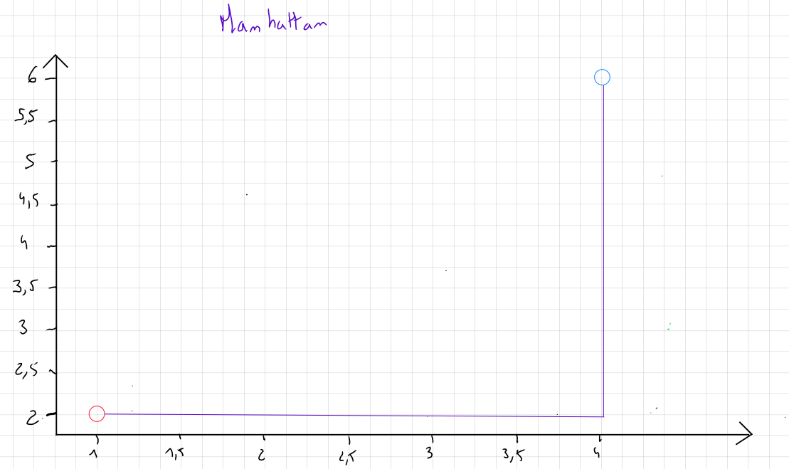
This measure is named after the distance a taxi travels on the streets of Manhattan, where all streets are either parallel or perpendicular to each other.

The formula for Manhattan distance is written as follows :

$$d(p, q) = \sum_{i=1}^{n} |p_i - q_i|$$

or

$$d(p, q) = |p_{i1} - q_{i1}| + |p_{i2} - q_{i2}| + \dots + |p_{in} - q_{in}|$$

For the following example :

ID	$x_1$	$x_2$	$x_3$	$x_4$	$x_5$	$x_6$	$x_7$	$x_8$
01	1.06	9.2	151	54.4	1.6	9.077	0	0.628
02	0.89	10.3	202	57.9	2.2	5.088	25.3	1.555

The distance is calculated as follows :

$$d_{1,2} = |1.06 - 0.89| + |9.2 - 10.3| + |151 - 202| + |54.4 - 57.9| + |1.6 - 2.2| + |9.077 - 5.088| +|0.628 - 1.555| = 61.286$$

The distance is calculated for all records $d_{1,3},d_{1,4},d_{1,...},d_{1,n}$

Minkowski Distance

Minkowski distance is a distance measure that generalizes both Euclidean and Manhattan distances.

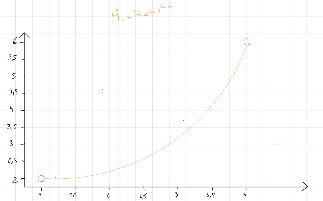
The formula for Minkowski distance is written as follows :

$$d(p, q) = \left( \sum_{i=1}^{n} |p_i - q_i|^p \right)^{\frac{1}{p}}$$

or

$$d(p, q) = (|p_{i1} - q_{i1}| + |p_{i2} - q_{i2}| + \dots + |p_{in} - q_{in}|)^\frac{1}{3}$$

$p$ is the power parameter that controls how differences between point coordinates are aggregated. This parameter can take various values, but common practice suggests using $p = 1$ ( which corresponds to Manhattan distance ), $p = 2$ ( which corresponds to Euclidean distance ), and values of $p > 2$, which are more sensitive to large differences between values.

In practice, Minkowski distance allows for testing different combinations by adjusting the $p$ value as needed.

For the following example :

ID	$x_1$	$x_2$	$x_3$	$x_4$	$x_5$	$x_6$	$x_7$	$x_8$
01	1.06	9.2	151	54.4	1.6	9.077	0	0.628
02	0.89	10.3	202	57.9	2.2	5.088	25.3	1.555

The distance is calculated as follows :

$$d_{1,2} = (|1.06 - 0.89| + |9.2 - 10.3| + |151 - 202| + |54.4 - 57.9| + |1.6 - 2.2| + |9.077 - 5.088| +|0.628 - 1.555|)^\frac{1}{3} = 3.94$$

The distance is calculated for all records $d_{1,3},d_{1,4},d_{1,...},d_{1,n}$

Defining the Value of K

The principle of KNN Nearest Neighbors is to define the final value based on the $k$ nearest neighbors, for example, the $3, 4$, or $5$ closest neighbors. However, this value is not chosen arbitrarily.

After calculating the distance between one record's values and the values of all other records, we must define a rule to specify to which class our record will belong ( classification ) or what the value of our record will be ( estimation ).

The simplest rule, which is the least complex in terms of computation, would be $k = 1$, meaning the value $y_i$ corresponds to the $y$ value of the nearest record. However, it turns out that the error rate is quite high in this case, and by convention, we define the rule: $k > 1$.

The idea is as follows :

1. Find the $k$ nearest neighbors of the record to be classified or estimated ;
2. Define the value based on a majority rule and threshold ( classification ) ; or a weighted average of the values ( prediction ) ;

Generally, if $k$ is too large, the model risks adjusting to noise, leading to overfitting. Bias is reduced, but variance increases. If $k$ is too small, we may not identify any structure in the data, reducing variance but increasing bias.

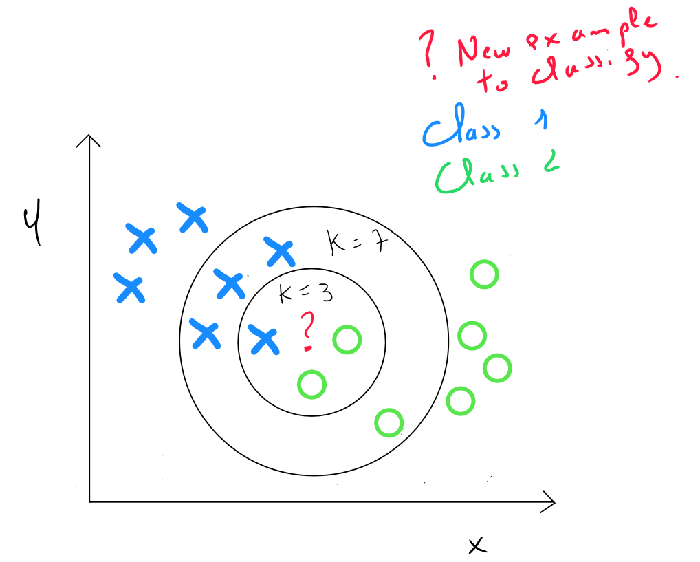
The choice of $k$ will focus on the value of $k$ that minimizes errors between $y$ and $\hat{y}$. Since KNN is a supervised technique, we use the training data, which is trained with several $k$ scenarios ( typically from $2$ to $9$ ), and select the value of $k$ that minimizes the model's errors.

The objective is to select $k$ that represents the best classification or estimation performance :

1. In classification, after training our model, we apply the model’s knowledge to the validation set and calculate the accuracy rate, i.e. the match between predictions and reality ( confusion matrix ) ;
2. In prediction, we perform the same operation, but then calculate the root mean square error (RMSE = √("MSE")) and select the $k$ that minimizes this sum ;

Defining ŷ

The algorithm will run a series of iterations on the training data, defining different values of $k$ to identify the $k$ that minimizes errors. Once we know the value of $k$, we still need to define a rule to determine the class or estimate the value.

Classification

For classification, the majority rule is directly related to the notion of a threshold. Suppose that for $k = 4$, $3$ values are "rich", and $1$ value is « poor ». In this case, our new record will correspond to « rich » because the probability that the value corresponds to « rich » is $75\%$ compared to $25\%$ for "poor". We typically define a threshold of $50\%$ to maximize accuracy.

Estimation

For estimation, we consider all the values of the nearest neighbors and calculate the predicted value based on the weighted average of the neighbors' values. The weighting is based on the notion of distance :

$$\frac{\sum_{i=1}^{n} w_i * x_i}{\sum_{i=1}^{n} w_i} \text{ where } w_i = \frac{1}{d_i} \text{ (} d_i \text{ = inverse of distance)}$$

Code Python KNN Estimation

import pandas as pd
from sklearn.datasets import fetch_california_housing


housing = fetch_california_housing(as_frame=True)


x = housing.data    #Predictors
y = housing.target  #House Price 

# Combining in a dataframe to display
data = pd.concat([x, y], axis=1)


data

# MedInc  = median income of households
# HouseAge = age of the house
# AveRooms = the average number of rooms per house
# AveRooms = the average number of bedrooms per house
# Population = the total population in area
# AveOccup =The average number of occupants per house
# Latitude
# Longitude
# MedHouseVal = Price (measured in hundreds of thousands of dollars

# Import libraries
import numpy as np
import pandas as pd
from sklearn.datasets import fetch_california_housing
from sklearn.model_selection import train_test_split
from sklearn.preprocessing import MinMaxScaler
from sklearn.neighbors import KNeighborsRegressor
from sklearn.metrics import mean_squared_error
import matplotlib.pyplot as plt

# Step 1: Split data into Train + Validation (60%) and Test (40%)
x_train_full, x_test, y_train_full, y_test = train_test_split(
    x, y, test_size=0.4, random_state=42
)

# Step 2: Split Train + Validation into Train (60%) and Validation (20% of total data)
x_train, x_val, y_train, y_val = train_test_split(
    x_train_full, y_train_full, test_size=0.25, random_state=42  # 0.25 x 0.6 = 0.15
)

# Step 3: Scale the data (KNN is distance-based and sensitive to scale)
scaler = MinMaxScaler()
x_train_scaled = scaler.fit_transform(x_train)  # Fit on train data
x_val_scaled = scaler.transform(x_val)  # Transform validation data
x_test_scaled = scaler.transform(x_test)  # Transform test data

# Step 4: Hyperparameter tuning using validation set
k_values = range(1, 21)
rmse_values = []  # Store RMSE for each k

for k in k_values:
    # Train the model with k neighbors
    knn_regressor = KNeighborsRegressor(n_neighbors=k)
    knn_regressor.fit(x_train_scaled, y_train)  # Train on training data
    
    # Validate the model on validation set
    y_pred_val = knn_regressor.predict(x_val_scaled)  # Predict on validation data
    
    # Calculate RMSE (Root Mean Squared Error) for validation set
    mse = mean_squared_error(y_val, y_pred_val)
    rmse = np.sqrt(mse)
    rmse_values.append(rmse)
    
    print(f"K={k}, RMSE (Validation)={rmse:.4f}")

# Step 5: Select the best K based on validation performance
best_k = k_values[np.argmin(rmse_values)]
print(f"Best K based on validation set: {best_k}")

# Step 6: Evaluate the final model on the test set
# Train the model with the best K on the training data
knn_regressor_best = KNeighborsRegressor(n_neighbors=best_k)
knn_regressor_best.fit(x_train_scaled, y_train)

# Predict on the test set
y_pred_test = knn_regressor_best.predict(x_test_scaled)

# Calculate RMSE for the test set
mse_test = mean_squared_error(y_test, y_pred_test)
rmse_test = np.sqrt(mse_test)
print(f"RMSE on Test Set (Best K={best_k}): {rmse_test:.4f}")


# Step 7: Visualize RMSE across different K values and include the test performance
plt.figure(figsize=(10, 5))
plt.plot(k_values, rmse_values, marker='o', label="RMSE (Validation)")
plt.axhline(y=rmse_test, color='r', linestyle='--', label=f"RMSE (Test) = {rmse_test:.4f}")
plt.title("KNN Regression: RMSE for Different K Values")
plt.xlabel("Number of Neighbors (K)")
plt.ylabel("RMSE")
plt.legend()
plt.grid()
plt.show()

# Step 8: Add a new data point for prediction
new_record = pd.DataFrame({
    'MedInc': [8.0],  # Median income
    'HouseAge': [30],  # Median house age
    'AveRooms': [6.0],  # Average number of rooms
    'AveBedrms': [1.0],  # Average number of bedrooms
    'Population': [500],  # Total population
    'AveOccup': [3.0],  # Average number of occupants per household
    'Latitude': [34.0],  # Latitude
    'Longitude': [-118.0]  # Longitude
})

# Scale the new data point
new_record_scaled = scaler.transform(new_record)

# Predict the house value for the new data point
new_prediction = knn_regressor_best.predict(new_record_scaled)
print(f"Predicted house value for the new record: €{new_prediction[0] * 100000:.2f}")

knn_regressor = KNeighborsRegressor(n_neighbors=best_k)
knn_regressor.fit(x_train_scaled, y_train)

new_x = np.array([[0.2, 0.5]])  # Example new X value (after scaling)
new_x_scaled = scaler.transform(new_x)
new_y_pred = knn_regressor.predict(new_x_scaled)
print(f"Predicted Y for new x={new_x} is {new_y_pred[0]:.4f}")

Code Python KNN Classement

# Load the Digits dataset
from sklearn.datasets import load_digits
import matplotlib.pyplot as plt
import pandas as pd

digits = load_digits()

# Features:
# Each sample has 64 features, representing the pixel intensities of an 8x8 grayscale image.
# Feature values range from 0 (white) to 16 (black).
x = digits.data  # Features (64 features per sample)

# Target:
# The target variable (y) represents the digit label (0 to 9).
y = digits.target  # Target labels (integers from 0 to 9)

# Shape:
# The dataset contains 1,797 samples and 64 features.
print(f"Shape of Features (x): {x.shape}")  # (1797, 64)
print(f"Shape of Target (y): {y.shape}")    # (1797,)

# Visualization:
# Each digit can be visualized as an 8x8 image.
# Below, we visualize the first sample in the dataset.
sample_index = 1  # Index of the digit to visualize
plt.figure(figsize=(4, 4))
plt.imshow(digits.images[sample_index], cmap="gray")  # Visualize the 8x8 image
plt.title(f"Digit Label: {digits.target[sample_index]}")  # Display the target label
plt.axis("off")
plt.show()

# Convert to DataFrame for easier exploration
# Each column represents a pixel (pixel_0 to pixel_63).
# The target column represents the digit label (0 to 9).
data = pd.DataFrame(x, columns=[f'pixel_{i}' for i in range(64)])
data['target'] = y  # Add the target column
print("First 5 rows of the dataset:")
print(data.head())  # Display the first 5 rows

# Import libraries
import numpy as np
import pandas as pd
from sklearn.datasets import load_digits
from sklearn.model_selection import train_test_split
from sklearn.preprocessing import MinMaxScaler
from sklearn.neighbors import KNeighborsClassifier
from sklearn.metrics import accuracy_score, classification_report, confusion_matrix
import matplotlib.pyplot as plt
import seaborn as sns


# Step 1: Split data into Train + Validation (60%) and Test (40%)
x_train_full, x_test, y_train_full, y_test = train_test_split(
    x, y, test_size=0.4, random_state=42
)

# Step 2: Split Train + Validation into Train (60%) and Validation (20% of total data)
x_train, x_val, y_train, y_val = train_test_split(
    x_train_full, y_train_full, test_size=0.25, random_state=42  # 0.25 x 0.6 = 0.15
)

# Step 3: Scale the data
scaler = MinMaxScaler()
x_train_scaled = scaler.fit_transform(x_train)
x_val_scaled = scaler.transform(x_val)
x_test_scaled = scaler.transform(x_test)

# Step 4: Hyperparameter tuning using validation set
k_values = range(1, 21)
accuracy_values = []

for k in k_values:
    knn_classifier = KNeighborsClassifier(n_neighbors=k)
    knn_classifier.fit(x_train_scaled, y_train)
    y_pred_val = knn_classifier.predict(x_val_scaled)
    accuracy = accuracy_score(y_val, y_pred_val)
    accuracy_values.append(accuracy)
    print(f"K={k}, Accuracy (Validation)={accuracy:.4f}")

# Step 5: Select the best K based on validation performance
best_k = k_values[np.argmax(accuracy_values)]
print(f"Best K based on validation set: {best_k}")

# Step 6: Evaluate the final model on the test set
knn_classifier_best = KNeighborsClassifier(n_neighbors=best_k)
knn_classifier_best.fit(x_train_scaled, y_train)
y_pred_test = knn_classifier_best.predict(x_test_scaled)

# Calculate Accuracy for the test set
accuracy_test = accuracy_score(y_test, y_pred_test)
print(f"Accuracy on Test Set (Best K={best_k}): {accuracy_test:.4f}")


# Step 7: Visualize Accuracy across different K values
plt.figure(figsize=(10, 5))
plt.plot(k_values, accuracy_values, marker='o', label="Accuracy (Validation)")
plt.title("KNN Classification: Accuracy for Different K Values (Digits Dataset)")
plt.xlabel("Number of Neighbors (K)")
plt.ylabel("Accuracy")
plt.axhline(y=accuracy_test, color='r', linestyle='--', label=f"Test Accuracy (K={best_k}) = {accuracy_test:.4f}")
plt.legend()
plt.grid()
plt.show()

# Step 8: Predict a new data point
# Create a new data point (an example 8x8 image)
# The pixel values should range between 0 and 16.
new_data = np.array([
    0, 0, 10, 14, 8, 1, 0, 0,
    0, 2, 16, 14, 6, 1, 0, 0,
    0, 0, 15, 15, 8, 15, 0, 0,
    0, 0, 5, 16, 16, 10, 0, 0,
    0, 0, 12, 16, 16, 12, 0, 0,
    0, 4, 16, 6, 4, 16, 6, 0,
    0, 8, 16, 10, 8, 16, 8, 0,
    0, 1, 8, 12, 12, 13, 1, 0
]).reshape(1, -1)  # Reshape to match the input shape (1, 64)

# Scale the new data point using the same scaler
new_data_scaled = scaler.transform(new_data)

# Predict the class for the new data point
new_prediction = knn_classifier_best.predict(new_data_scaled)
predicted_label = new_prediction[0]  # Predicted digit label

print(f"Predicted digit for the new data point: {predicted_label}")

# Visualize the new data point
plt.figure(figsize=(4, 4))
plt.imshow(new_data.reshape(8, 8), cmap="gray")  # Reshape to 8x8 for visualization
plt.title(f"Predicted Label: {predicted_label}")
plt.axis("off")
plt.show()