Anomaly Detection

Anomaly detection is an unsupervised technique where learning consists of examining a dataset considered to represent normal events in order to detect an abnormal event.

note

Some of the diagrams and concepts presented here are inspired by the Machine Learning course by Andrew Ng, a program created in collaboration between Stanford University Online Education and DeepLearning.AI, available on Coursera. Find the original course here: Machine Learning by Andrew Ng.

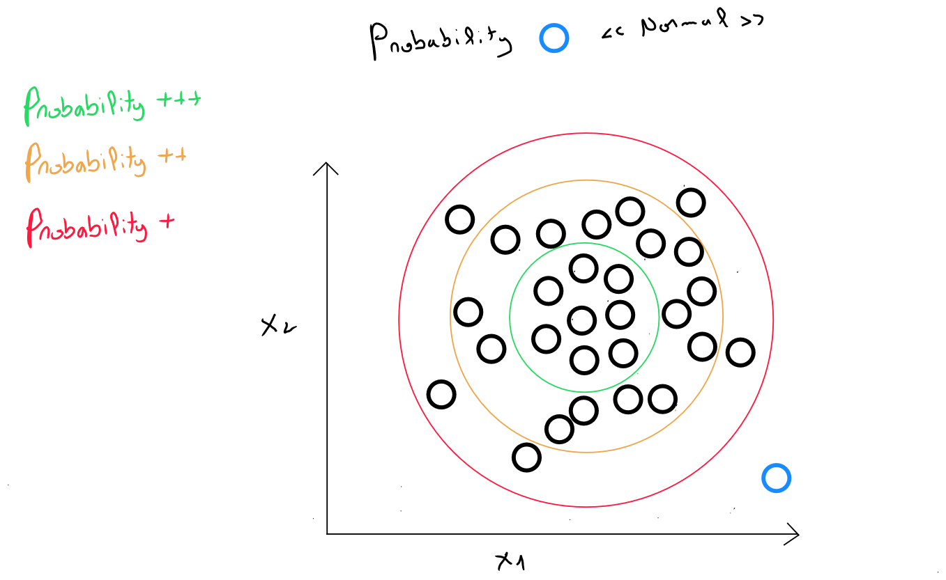
Take the example of a factory that produces airplane engines, where the final test involves running each engine and measuring the vibrations and temperature.

We have two variables $x$ : $x_1$ generated heat and $x_2$ vibration intensity, as well as values for all the tests performed on engines considered to be normal.

We have values for a new record $\textcolor{blue}{x_{test}}$.

The idea behind anomaly detection is to determine whether the new engine's data is similar to the data from previously manufactured engines.

For anomaly detection, we have data : $x^{(1)},x^{(2)},...,x^{(n)}$, and our model can be considered as the probability that new values exist within the « correct » data.

Anomaly detection works based on the Gaussian approximation principle. Essentially, this means that even if the data is not perfectly Gaussian, it can be approximated by a Gaussian distribution - at least for the majority of records - and anomalies are defined as points that are far from this majority.

Gaussian Distribution

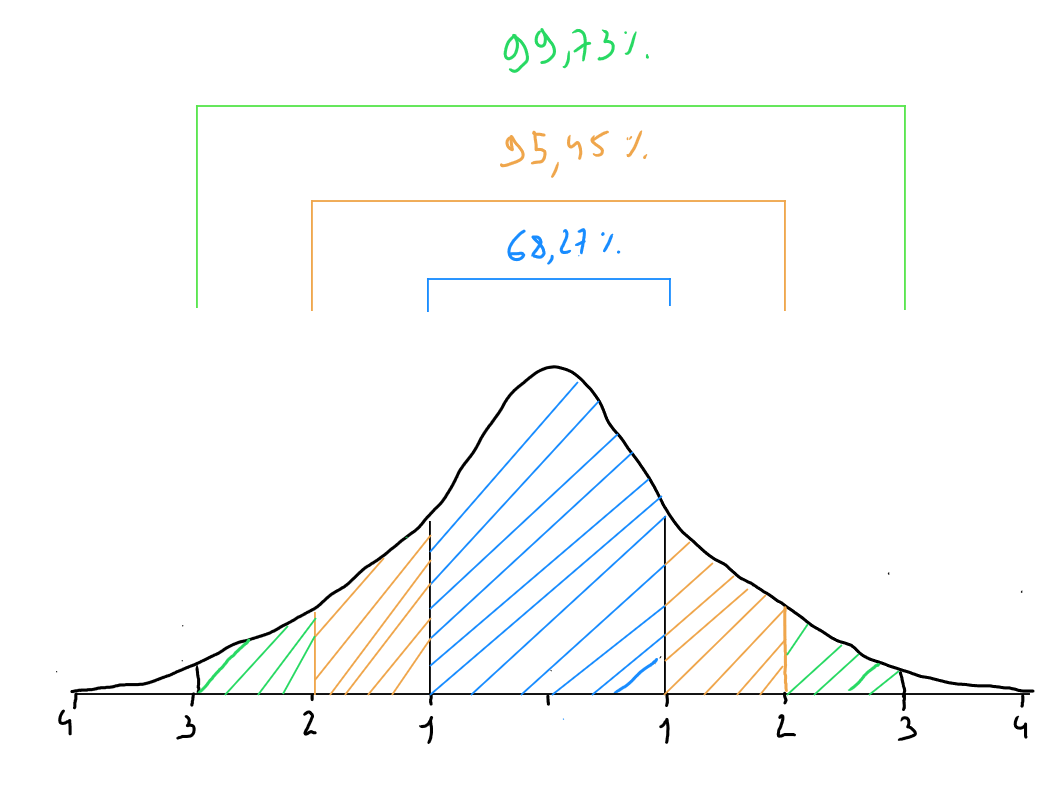
A Gaussian distribution, also known as a bell curve, is symmetric around its mean. The mean defines the center of the distribution on the x-axis ( where the peak of the curve is located ), and the variance measures the dispersion of the data around the mean.

In a Gaussian distribution, the mean corresponds to both the mode and the median ( perfectly symmetric curve ).

As we discussed in the section on univariate statistical principles, variance measures the spread of values in a variable. It is calculated as the average of the squared differences from the mean and is always positive.

Variance is calculated as follows :

$\sigma^2 = \frac{\sum_{i=1}^{N} (x_i - \mu)^2}{N}$.

In a Gaussian distribution, the following empirical rule applies :

• $68.27$ of the data is within one standard deviation of the mean ;
• $95.45$ of the data is within two standard deviations of the mean ;
• $99.73$ of the data is within three standard deviations of the mean ;

Probability Density of a Normal Distribution

The probability density of a normal distribution indicates the relative probability that $X$ takes a value within a small interval around $x$. Capital $X$ represents all possible outcomes of a variable, and lowercase $x$ is a specific value that $X$ can take. In other words, the probability density indicates how likely a random value is to be near another value.

The probability density formula for a normal distribution is :

$$f(x; \mu, \sigma^2) = \frac{1}{\sqrt{2\pi\sigma^2}} \exp\left(-\frac{(x - \mu)^2}{2\sigma^2}\right)$$

Where $\pi$ corresponds to $3.141592653589793$ and $sigma^2$ is $\frac{\sum_{i=1}^{N} (x_i - \mu)^2}{N}$.

This probability density has the following properties :

• The sum of probabilities for all possible values of $x$ equals $100$ ;
• The density is symmetric around the mean $𝜇$. The probability is highest near $𝜇$ and decreases as $𝑥$ moves away from $𝜇$ ;
• The tails of the distribution, representing extreme events, decrease very rapidly ;

Probability Densities of $𝑛$ Different Features

In real-world anomaly detection, we deal with a record containing values for multiple variables. This means we're working with a multivariate distribution ( not univariate ). An anomaly may consist of a record in which some variables are consistent with the norm, but one particular variable is abnormal. To detect this abnormality, it's important to consider the independence of features and calculate the individual probability densities for each variable in a normal distribution, then multiply them together.

In practice, this involves applying the following formula :

$$p(\mathbf{x}) = p(x_1; \mu_1, \sigma_1^2) \times p(x_2; \mu_2, \sigma_2^2) \times p(x_3; \mu_3, \sigma_3^2) \times \dots \times p(x_n; \mu_n, \sigma_n^2)$$

This can be rewritten as :

$$\prod_{j=1}^{n} \frac{1}{\sqrt{2\pi\sigma_j^2}} \exp\left(-\frac{(x_j - \mu_j)^2}{2\sigma_j^2}\right)$$

We have values for a new record $\textcolor{blue}{x_{test}}$ to which we apply our formula.

The rule is as follows :

• If $\textcolor{blue}{x_{test}}$ < $𝜀$ (a very small number), then
  anomaly ;
• If $\textcolor{blue}{x_{test}}$ >= $𝜀$, then
  normal ;

We define a threshold $𝜀$ ( epsilon ) to classify a record as normal or anomalous based on the probability density formula of $n$ features. $𝜀$ is a very small number, assuming that $99.73$ of the data is within three standard deviations of the mean.

Defining the Threshold $𝜀$

To define $𝜀$, we split our data into a training and validation set. While this may resemble a supervised technique, a supervised technique would not be effective because anomaly detection typically involves very few « anomaly » cases, making it difficult for a parametric or non-parametric algorithm to predict accurately.

Let's consider the following example : we have 10,000 records containing values for manufactured airplane engines that showed no anomalies, and 20 records ( 20 engines ) for which anomalies were detected.

In this case :

1. We split the data and train our model on 8,000 « normal » records. Training consists of calculating the Gaussian probability density for each record ($x$) ;


2. We then sort these probabilities in descending order and select several $p$ values ( Gaussian probability density ) among the lowest ones ;


3. These values are tested as the threshold $𝜀$ ( epsilon ) on the remaining 2,000 validation records ( including 20 anomalies ), and we identify the value of $𝜀$ that best distinguishes between anomalies and normal data without classifying normal data as anomalies ;

Feature Selection

So far, we have seen that our algorithm performs the following steps :

1. Select $n$ features : $\vec{x} = [x_1, x_2, ..., x_n]$ ;


2. Calculate parameters $\mu_1, ..., \mu_n, \sigma_1^2, ..., \sigma_n^2$ ;


3. Given a new record for $x$, calculate $p(x)$: $p(x) = \prod_{j=1}^{n} p(x_1 ; \mu_1, \sigma_1^2)$ or $\prod_{j=1}^{n} \frac{1}{\sqrt{2\pi\sigma}} exp^{-\frac{(x-\mu)^2}{2\sigma^2}}$ ;


4. Result = if $p(x) \leq \epsilon$, anomaly; if $p(x) > \epsilon$, normal ;

One key condition is to have Gaussian-distributed variables. This condition is not always met, and there are ways to improve a distribution to make it more Gaussian :

• $np.log(𝑥_1+0.001)$ ;
• $np.log(𝑥_1+1)$ ;
• $np.log(𝑥_1+2)$ ;
• $np.log(𝑥_1+3)$ ;
• $x_1 = \sqrt{x_1}$ ;
• $x_1 = x_1^{1/3}$ ;

Code Python

import numpy as np
import pandas as pd
from scipy.stats import norm
import matplotlib.pyplot as plt

#Synthetic data
np.random.seed(0)
x1 = np.random.normal(50, 10, 8000)  # 8000 correct records x1  - average 50 ; standard deviation 10
x2 = np.random.normal(30, 5, 8000)   # 8000 correct records x2  - average 30 ; standard deviation 5

# 2000 validation records (1980 normal, 20 not normal)
x1_val = np.random.normal(50, 10, 1980)
x2_val = np.random.normal(30, 5, 1980)

x1_val_anomalous = np.random.normal(80, 5, 20)  
x2_val_anomalous = np.random.normal(10, 5, 20)  

x1_val = np.concatenate([x1_val, x1_val_anomalous])
x2_val = np.concatenate([x2_val, x2_val_anomalous])

train_data = pd.DataFrame({
    'x1': x1,
    'x2': x2
})

val_data = pd.DataFrame({
    'x1': x1_val,
    'x2': x2_val,
    'label': [0]*1980 + [1]*20  # 1 = Anomaly
})

mu_x1, sigma_x1 = np.mean(train_data['x1']), np.std(train_data['x1'])
mu_x2, sigma_x2 = np.mean(train_data['x2']), np.std(train_data['x2'])

def gaussian_probability_density(x, mu, sigma):
    return (1 / (np.sqrt(2 * np.pi) * sigma)) * np.exp(-0.5 * ((x - mu) / sigma) ** 2)


train_data['p_x1'] = gaussian_probability_density(train_data['x1'], mu_x1, sigma_x1)
train_data['p_x2'] = gaussian_probability_density(train_data['x2'], mu_x2, sigma_x2)
train_data['p'] = train_data['p_x1'] * train_data['p_x2']

val_data['p_x1'] = gaussian_probability_density(val_data['x1'], mu_x1, sigma_x1)
val_data['p_x2'] = gaussian_probability_density(val_data['x2'], mu_x2, sigma_x2)
val_data['p'] = val_data['p_x1'] * val_data['p_x2']

epsilons = np.linspace(min(val_data['p']), max(val_data['p']), 1000)
best_epsilon = None
best_f1 = 0

for epsilon in epsilons:
    predictions = val_data['p'] < epsilon
    tp = np.sum((predictions == 1) & (val_data['label'] == 1))
    fp = np.sum((predictions == 1) & (val_data['label'] == 0))
    fn = np.sum((predictions == 0) & (val_data['label'] == 1))

    if tp + fp == 0 or tp + fn == 0:
        continue

    precision = tp / (tp + fp)
    recall = tp / (tp + fn)
    f1 = 2 * precision * recall / (precision + recall)

    if f1 > best_f1:
        best_f1 = f1
        best_epsilon = epsilon

print(f"Best Epsylon found: {best_epsilon}")
print(f"Best F1 Score: {best_f1}")

val_data['anomaly'] = val_data['p'] < best_epsilon

print(f"Detected anomaly: {val_data['anomaly'].sum()} sur {len(val_data)} enregistrements de validation")

plt.figure(figsize=(10, 6))
plt.scatter(val_data['x1'], val_data['x2'], c=val_data['anomaly'], cmap='coolwarm', marker='o')
plt.xlabel('Température (x1)')
plt.ylabel('Vibrations (x2)')
plt.title('Anomalies detection')
plt.show()